A typical plot of an ocean track is shown below using the default scale of 60 nmi per printed latitude parallel. The longitude scale is set up using the inserted diagram, after marking the central Lat on the Lon scale of the diagram.
An ocean voyage proceeds as a sequence of fixes with DR between them. These real sextant sights are from our book Hawaii by Sextant. We will be looking specifically at Problem 22, which is zoomed into below.
This is a good fix, but we can't tell how good using the standard scale for the plots shown here. We can expand the standard scale by redefining the Lon diagram. Below is how it would change if we go from 60 nmi per parallel to 30 nmi per parallel.
Or we can expand the plots to 6 nmi per parallel as shown below.
This is the type of expansion we used in practice during the 1982 voyage shown above. A typical procedure might be to do a quick fix with just two or three sights to find an approximate center point, and then create the new plotting sheet centered about that point using 6 nmi per parallel.
At the time of the voyage, we chose 24º 39'N, 151º 16' W to plot from, and below is an image of the actual plotting sheet from that voyage, 37 year ago.
You can see that we had a good fix. Refer to Hawaii by Sextant to review our Fit Slope Method in action along with our automated LOP advancement technique, which is required for best accuracy. This makes a set of 15 sights of four bodies an extended running fix over a 30 minute sight session to get equivalent sights at one time. Both yield notable improvements to the multiple sights analysis. In this sight session, Capella was the weakest with just one sight; the other three had at least 4 each.
Here is a short video discussion of the above process:
We usually try to get all of the GRIB files we need from within the navigation program or GRIB viewer we are using. This solves a key issue of being sure that the ones they let us request will indeed be viewable in their viewer. All such sources of GRIB data offer a filter for Lat-Lon region and desired parameters, as well as resolution, and time intervals and duration (ie every 3h out to h72).
Some navigation programs, such as Expedition, have many of the top model products coded into their system so there is less reason for getting external data, others have limited products, and it is not uncommon that popular charting software might only offer GFS parameters internally, maybe with the addition of RTOFS for currents and WW3 for waves.
The popular OpenCPN can create email requests to Saildocs, but the packaged interface options do not include many important models Saildocs offers. OpenCPN can view some grib2 files, but not all. Some of the new high-res data come in a Lambert projection which takes new programming. There are also new parameters to be included. The forthcoming version of OpenCPN (newer than present 5.0.0+9065270) will include simulated radar (composite reflectivity, REFC), which is available in several WRF models, as wells as the NBM, and now globally in the new GFS version that came into effect on June 12, 2019.
REFC is not yet available as part of a GFS request to Saildocs, but we have other ways to get the data underway from Saildocs, as shown below. I understand that REFC will be added as a request parameter in XyGrib in July or August. XyGrib will show the files if you get them elsewhere, i.e., as outlined below. It is already available in the European WRF models from https://openskiron.org/en/. We can also get this parameter from several models using LuckGrib, and then export the file to be loaded into a navigation program. LuckGrib has the high-res regional versions of REFC as well as the global.
Sample of REFC over SW Pacific viewed in LuckGrib
The notes below go beyond the new REFC parameter and show how to request GRIB files in general directly from their primary source, NCEP. The link we start from is:
The procedure is outlined below, followed by a video link demonstrating the process.
Step 1. The main link takes you to a list of many models, with various ways to access the data. We want to use here the "grib filter." The header name is also a link to the process we are outlining here. The other data sources are huge files of global coverage and hundreds of parameters.
Step 2. Choose a model. For now we will use GFS 0.25 degree. This is now the new GFS, and it will as of yesterday include the RECF. Click "grib filter" for that one.
Step 3. This takes us to an index of data files, and we note (at least for now) that there is a format change yesterday when the new GFS went online. We have to choose one newer than 20190613. This is yyyymmdd. We choose 20190614.
Step 4. The next page shows the synoptic time computations: 00, 06, 12, 18. Normally we would want the latest model run. Let's say the latest is 12z. That will be the top one on the list. Some hours after 18z, the 18z file will appear at the top of the list. (More on time delays and latency later on.)
Step 5. Now we are on the request page, where we select, valid forecast time, parameters, levels, and Lat-Lon region. At every synoptic time, there will be 364 forecasts made. Let's assume we want every 6h starting at the 12z run for the next 24h. Thus we want 12zf000, 12zf006, 12zf0012, 12zf0018, and 12zf0024. This is 5 files and we have to ask for these individually.
Parameters
Let's say we want wind, pressure, and simulated radar. We could get others, as discussed below.
For the wind we ask for UGRD, VGRD, which are the E-W and N-S components of the wind; the grib viewer will make these into a wind vector.
For the Simulated radar we ask for REFC
For the pressure we could ask for PRMSL, which is the common one used, or we could ask for MSLET, which is actually a more precise pressure parameter, but some grib viewers might not be set up to recognize this. We do not want PRES, which is a parameter used for weather on land.
Other useful parameters are discussed below.
Levels
For wind we need "10 m above the ground." For PRMSL we need "mean sea level." For REFC we need plain "entire atmosphere" and not "entire atmosphere (considered as a single layer)."
Step 6. After selecting a file, parameters, and levels—you will see online that they present this in a different order—put a check in the box "Make a sub region" and then enter the bounds. Lon West is negative (-); Lat South is (-). We will get Cape Verde region for a small sample, -30 to -14, and 20 to 10.
Step 7. Put a check in the Box "Show URL only for web programming," then press enter and you will get this link:
URL= https://nomads.ncep.noaa.gov/cgi-bin/filter_gfs_0p25.pl?file=gfs.t12z.pgrb2.0p25.f000&lev_10_m_above_ground=on&lev_entire_atmosphere=on&lev_mean_sea_level=on&var_PRMSL=on&var_REFC=on&var_UGRD=on&var_VGRD=on&subregion=&leftlon=-41&rightlon=-16&toplat=40&bottomlat=26&dir=%2Fgfs.20190614%2F12 If you are on land with an internet connection, you can then take away the "Show URL..." check mark, then when you press Download you will get the file called:
gfs.t12z.pgrb2.0p25.f000
At this stage you might want to add a .grb to the file to get gfs.t12z.pgrb2.0p25.f000.grb, then you know what you have, but this is not necessary. We have shown that both OpenCPN and XyGrib will open the files as downloaded without the .grb added, or with it.
This file will then load into OpenCPN, but you won't see the REFC until the next version of OpenCPN. The latest version at the moment (5.0.0+9065270) does not have the REFC implemented in the GRIB plugin, but the developers have it working in the next version, as shown in the video.
To get these files from Saildocs when underway you would send a mail to query@saildocs.com with the message being
You could request as many as you like. These are about 56 kB each as returned by regular email (~twice actual size). Using special satcom email they could get reduced quite a bit. They will come back as individual emails with the files attached. The video below shows how to get these by email, and then view them in XyGrib and in a forthcoming edition of OpenCPN, along with some discussion of this new REFC parameter. With this method of requesting specific parameters and levels, navigators may also find it useful to look into the 850 mb level for both wind and relative humidity (RH). This is the boundary layer level at about 1000 m, where the winds become less, if at all, affected by surface friction. About the altitude of low clouds. These winds are a good indication of the direction of squall motion (compare with REFC forecasts), and in the tropics, the streamline view at this elevation can give indication of wind flow on the surface that does not show up in the actual wind data. We watched a prominent example of this off the coast of Queensland, AU earlier this month. The RH at this level can also show a good outline frontal systems, which are not always easy to discern from wind and pressure. ____________________ To obtain a HRRR CONUS wind and pressure (surface analysis, h0 forecast = f00) on Feb 4, 2020 at 18z from saildocs, it would be:
send https://nomads.ncep.noaa.gov/cgi-bin/filter_hrrr_2d.pl?file=hrrr.t18z.wrfsfcf00.grib2&lev_10_m_above_ground=on&lev_mean_sea_level=on&var_MSLMA=on&var_UGRD=on&var_VGRD=on&subregion=&leftlon=-131&rightlon=-120&toplat=42&bottomlat=33&dir=%2Fhrrr.20200204%2Fconus Adjust Lat, Lon and times as needed ____________________
Video demo of getting the files.
Video demo of viewing REFC in XyGrib.
Video demo of viewing REFC in OpenCPN.
On the list is to add a video devoted to the practical use of REFC and data we have to confirm it... which is easy to test because we have archived real weather radar online.... and you can go to squally waters in real radar view, forecast some pattern and then see if it pans out.
We also want to add a short article and video note on use of the 850 mb data, as outlined above, which you can obtain with the methods outlined here.
Well... that's a bold statement; let's clarify. First, I am speaking of charts that are equivalent to official charts, as opposed to 3rd party charts, such as Navionics or Garmin Blue charts, among others. Both of these can be good in some areas; both can be bad in some areas. Sometimes these limitations are not just the chart, but the chart viewer. In most cases, these chart companies control the viewers, but some platforms are more versatile than others. Once these proprietary charts are then sold or licensed to other companies, more issues can arise, as they might, for example, license only some scale levels and not others. There have been notorious accidents traced at least in part to that issue. But none of that matters here. We can use paper charts or electronic charts (echarts), but for a "deal," we would have to mean echarts, because all paper charts are expensive, and rarely on special. Also of course, by "international" I mean waters other than the US waters, because all US echarts are free—the obviously best deal. A few other nations also offer free echarts for some of their waters (see charts section at OpenCPN). Echarts come in two formats: raster navigational charts (RNC), which are graphic images of the paper charts, and vector charts, which are all digital data; the chart display is created from numerical parameters by the nav app as we view it. Vector charts can in principle include much more information than possible with raster charts, such as Light List and Coast Pilot data, as well as more descriptive attributes of the various charted objects. The bargain here is with the vector charts, because they are smaller files than RNC, and they are notably easier to maintain, manage and distribute, not to mention having the potential to include more information. All maritime nations make a set of vector charts in the official IHO standard called S-57. These are called electronic navigational charts (ENC). The third party charts mentioned above are all "vector charts," but they are not ENC, and therefore not official charts. To understand this "best deal ever" we need to look a bit more into how ENC are displayed in navigation apps, which is outlined below, but I should mention that we have a book on the design and use of ENC charts that includes all the practical detail needed to take advantage of the powerful ENC resource, as well as explaining relative roles of RNC and ENC. It also includes tips on use of echarts in general.
"Great book! I wish I had had this resource many years ago when just starting to craft OpenCPN. Would have saved me lots of effort pulling together the sometimes baffling set of standards and connected parts that is the current ENC landscape. Especially, having ENC Chart 1 available in clear color printed form is a huge benefit. And the annotations are a bonus. Well done! I will heartily recommend this volume to OpenCPN users as the opportunity presents."
—Dave Register, originator and lead developer of OpenCPN.
ENC products must include all the information specified in the IHO S-57 standard, but that standard does not tell us how the data should be displayed to the navigator. The display of the data is specified in IHO S-52 standard, and any navigation app or system that hopes to be certified "Type Approved" must meet the S-52 display standard—and indeed several other factors having to do with interface, chart updating, and back-up. In passing, the ENC display in OpenCPN is as good as any we have seen outside of type approved apps, and indeed some of the choices made in OpenCPN that are not strictly standard could be considered an improvement by many navigators. The developers at OpenCPN have been very good about making improvements in the display whenever needs are detected. The common factor among all nav apps capable of showing ENC, whether or not they are type-approved, is the way they process the chart files. Upon initial install, they load the standard ENC file issued by the producing Hydrographic Office, and the first thing they do is convert the ENC files to a format they can read and display efficiently in their own system, and then they store this new file on the hard drive along with the original ENC. The new file is called the System ENC, or SENC file. A SENC file is some 2.5 to 5 times larger than its base ENC, depending on the nav app and individual charts. Thus every navigation app running official ENCs will have two copies of the chart installed. The government ENC and their own unique SENC file. The ENC files of a specific chart are the same loaded into any nav app, but the SENC files created in that app are unique to that specific nav app. Other than from the US and a few other nations offering free ENC in S-57 format, most maritime nations package their ENC into an encrypted format called IHO S-63. This is basically a protective envelope they wrap around the ENC, whose content is still determined by S-57. OpenCPN has a plugin to allow for the display of S-63 (ENC) charts, but these charts are not the subject at hand now. The S-63 official charts are all fairly expensive. Since international ENCs are encrypted (for copy protection and to guarantee accurate data), you cannot even create a SENC file without having needed credentials on your computer, which typically include some form of a fingerprint of your computer system along with a chart serial number that is proof of purchase of the chart. Therefore it is no surprise that you cannot just copy the SENC file of a chart and send it to a friend using the same navigation app. The IHO has, however, approved the distribution of SENC charts that have been created by licensed providers, but these charts may not be referred to as "official charts," and indeed as such would not meet carriage requirements. They do this in part to protect their official chart sales, but also because they did not make the actual charts themselves and therefore cannot guarantee that the charts are indeed identical to the official ENC, nor can they guarantee that the update system works as intended. The special deal on international charts referred to here are SENC charts produced specifically for OpenCPN by o-charts.org, a company of sailors in Barcelona. Since every nation has their own regulations on the use of their SENC charts, the License agreement from o-charts lists them all. Not all nations offer this SENC option, but many do, and this does indeed look like the future of electronic charting. It has the advantage of being a machine language file that runs fast, and takes up half the space of a native ENC installation—and as we see here, companies have the option of providing these at very economical costs. I must also add, another thing that contributes to them being the "best deal" in charts is that they are made for OpenCPN, which is a topnotch nav app. There are several very good commercial nav apps, but there are others that are not very good. Had one of the poor products offered the SENC charts it would not be such a good deal. As noted below, there are indeed international charts that cost less.
The limits on the SENC charts are they are unique to the navigation app they are made for, and second, they are not "official charts." The providers (o-charts) can and do state that the charts are identical to the latest official versions, and they include free updates for some period of time, typically one year. The SENC charts we have tested have indeed been identical to official ENCs, and the update process works well. The primary reference for ENC and SENC related matters is the excellent IHO Pub. S-66 Facts About Electronic Charts and Carriage Requirements (SENC is on pages 13 and 31-34). So with that long introduction, the deal we are discussing here are SENC charts made for OpenCPN, available from o-charts.org. This company is licensed by the nations that offer a SENC option. They produce the SENC chart files for OpenCPN (called 0eSENC, OpenCPN encrypted SENC) and then they sell and distribute these oeSENC directly to us without any interaction with the primary ENCs. One year of free updates is included. Nations update on different schedules. We have tested this system, and it works well. Easy and efficient. And indeed a deal! You can, for example, buy all of the charts of Australia (889 charts!) for 35 euros (~$40). The ENC cost is about $580. The international selection of oeSENC charts available is given here. For comparison shopping, o-charts offer all of West Coast Canada (BC) for 20 euros. The ENCs from Canada are some $1,200!; the best previous bargain I knew of was Rose Point price of $99, but they can only be used on their nav app Coastal Explorer (these are S-63 not SENC), which is an excellent navigation program but is costs $365. Rose Point does have the BC raster charts for $99 as well, again restricted to Coastal Explorer. O-charts says they are working on raster versions as well, but that is a big project... recall the notes above on why vector charts can be a bargain. In further contrast, I must note for completeness that the least expensive of all electronic chart options are the Navionics apps for mobile devices, and in this case the one called "Boating US & Canada." That is just $22 for nav app and charts for all US and Canadian waters, but the charts and app both have notable limitations. It would be stretching the point to call its use navigation... it is, as they describe it, "boating." To be fair, however, very many prudent navigators have in fact used the Navionics charts in one form or the other around the world, for short and long passages. But they have to be on top of things at all times, to deal with anomalies that might show up.
I am using OpenCPN 5.0 on a Mac, but users should double check that any crucial plugins they want to use are available for ver 5.0 on the Mac. At this moment, the Mac plugins are in process. All the standard plugins work for the PC ver 5.0. As it might be called for, there are multiple ways to run the PC version of OpenCPN 5.0 on a Mac, which I will review in another article. Several are free; others have just a modest cost. The license you purchase from o-charts.org allows for two "installations," where each installation identifies the computer and its operating system. If you update your OS it will look like a new computer and you will have lost one install. Thus we have to think carefully on these matters. An alternative approach available only to PCs at the moment is to purchase a dongle from o-charts for 19 euros, and then one of the "installs" can be assigned to the dongle. This does not put the charts on the dongle, just your registration credentials for specific charts. Then you can plug the dongle into any PC or OS to make that system a legal viewer, but now it can be moved from one system to another. The system would of course have to be running a copy of OpenCPN, 4.5 or newer.
To use these SENC charts from o-charts you will need the free oeSENC plugin for OpenCPN. It is a simple install and the process of buying the charts and then creating the fingerprint is straight forward. I am going to order a dongle (total of 23 euros ~$26) to ship to the US. Then I will purchase the Canadian BC charts and make a video of the full process to add here. In the meantime, there is an excellent video on the step-by-step process of obtaining and installing these charts made by o-charts.
There is no audio with the video, but that is not needed. It shows clearly every step. Keep in mind the OpenCPN is an international product, with more language versions than any other navigation app, so no one language meets all needs in the demos. This video does not include the step of building and using the fingerprint file, but that is covered in the articles below. ...and somewhere down the line we do have to make our promised video series on the use of ENC, because ENC are not plug and play. They include much more info than raster or paper charts, but it takes a new approach to chart reading to take advantage of them, which our book above provides. Thus it is important that you know the type of chart you are getting and how to use them. You can download and work with the US versions (see starpath.com/getcharts) to see how they function, but our text on echarts (above) would help a lot with this (there are Kindle and Apple Books as well as paper). If you do not have that book, this reference from Claris on ENC objects and attributes will be helpful. This Russian version has a different format for the same data (www.s-57.com)—if the two differ, the Claris cite is more likely to be up to date.
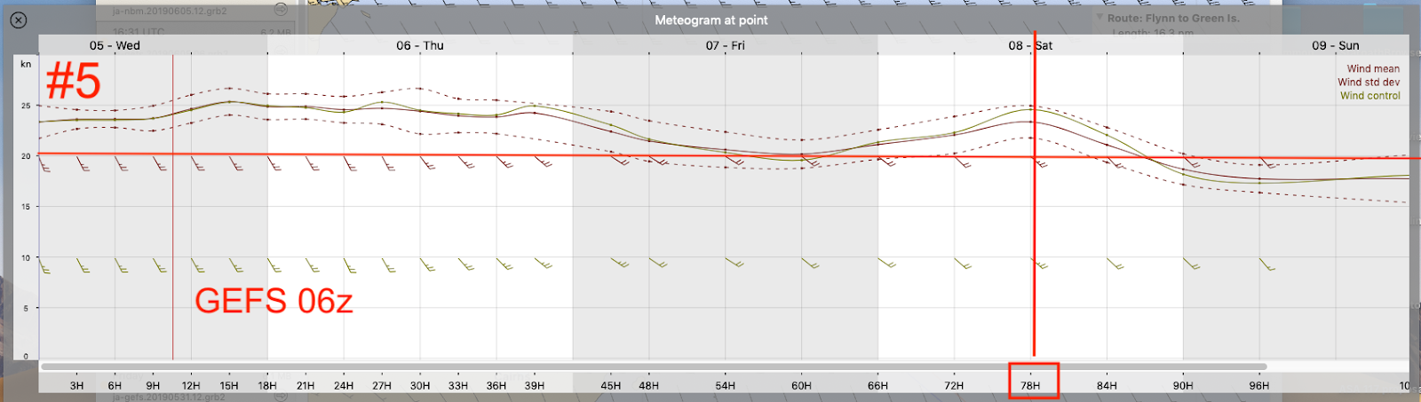
We recently completed a comparison of several models looking for the best extended forecast. The apparent winner in that case was the NBM. There are arguments on why this might in fact be expected to be best for extended forecasts; we will come back to that. For now we have another, equally crucial test at hand. And in this case it looks like an ideal way to make this test, because the NBM is notably different at 78 hr out than the "competitors," namely GFS, FV3-GFS, and GEFS, and to the best we can estimate it, the ECMWF. The vessel we are following is moored off of Flynn Reef in the Great Barrier Reef, 30 nmi east of Cairns in Queensland. He needs winds solidly less than 20 kts to make progress on the last leg of his 9,000 mile row (actual miles rowed, not great circle) from Neah Bay, WA to Cairns AU. We will use Sat Jun 8, 12z as our test point, which is 78h from the most recent model runs at 06z Wed, Jun 5. Below are the meteograms for this period at that location that we obtain from LuckGrib. Note: you can click one of these to zoom it, then subsequent clicks takes you through the set.
The above is our guess of the ECMWF from windy.com. The 3 AM shown is AU local time; add 10h to 12z to get local time = 22 LT. We will add more forecasts, every 12 hr or so. to see how things evolve. For the moment, we would not have confidence to recommend chances of wind well below 20 on Fri / Sat, but that might change.
========== The next day: Thursday Jun 6==========
Jacob needs winds well below 20 (~ 15 or so) from the SE, or he can also make progress to the west with winds of 20-25 if the direction is more easterly, that is ideally due east (090) or as far south at 110 to 120 at the lighter end of the speeds. So far all forecasts are 20-25 at SE or even more southerly, which is no go.
Below is the NBM meteogram for Jacobs present position
The test case we are following here is on Sat, but that wind, even if it pans out, is not a go situation. On the other hand, we see some indication of winds going more easterly on Friday (tomorrow), still strong however. The Cairns forecast for now also has indication of going a bit easterly on Friday... whereas all other forecasts now for before or after friday is the ole 20-25 going to 30 at SE.
Friday 7 June
Strong Wind Warning for Friday for Cairns Coast
Winds
East to southeasterly 20 to 25 knots, reaching up to 30 knots offshore at times.
We also get this indication of some more easterly from the FV3
A narrow window tomorrow. This moment is just before daylight on Friday, so we will pass on this info to see what it looks like on the water.
----- added 04z Jun 9-------
In retrospect he did take off Friday, and indeed did get to Cairns, but it was a long hard row. We have not heard from him since arriving, but we do know the winds in the region from Cairns observations shown below.
The NBM from 84 hr out called for 21 from the SE, the actual winds were 23 or so. This is about as close as we could want. In this case the FV3 and the GFS were both over 25, also from SE, so this is not such a conclusive distinction between NBM and FV3 GFS. On the other hand, a more subtle and encouraging verification is the wind did indeed back around to the east on Friday and called for in NBM and FV3, and that was what triggered Jacob to leave. The wind did not at all go lighter and we are not sure of the direction at the boat, but it was a long tough row to get to cairns.
On June 12, the GFS will be updated to the new FV3-GFS, which promises to be a big improvement in global forecasting. We have been following the winds off the coast of Queensland, Australia in a real world example of needing the best possible long-range forecast. See Tools for Crucial Weather Routing: With an ongoing comparison of GFS and FV3-GFS. This note here is a summary of those results, which we can do now that we know what the winds turned out to be. We started with a 90h forecast, using Friday May 31 at 12z as our test case. The boat was travelling at about 1.5 kts at the time, so the location did not effectively change relative to ocean wind patterns. But we see that at that location, the wind did indeed change a lot with time, so we stick with our 12z reference. Below are the winds for that day and location. Observed wind from Emerson on Fri May 31 located 154 nmi from Cairns, in direction 123T. 00z to 08z 12 @ 070 08z to 14z20 @ 130-140 14z to 20z15 @ 130-140 20z to 00z20 @ 130-140 This location is 10h ahead of UTC, so the local times are 10h later than those shown. Here is a summary of the results, keeping in mind the right answer is SE 20.
It is difficult to see any systematic behavior amongst this data—the meteograms in the original post might help with that. It was a difficult situation to forecast, because the isobars off the NE coast of AU (Queensland) were affected by a huge ridge about a big High in the Bight at the southside of AU. The isobars moved around as this big high moved, and they were also influenced by fronts to the east of AU. Except for a poor start on the speed at 90h, the FV3 did overall better than the GFS it will soon replace. That is good news. We would have to call the Oceanic National Blend of Models as the winner of best extended forecasting. It includes the ECMWF, and after June 12 will likely include the FV3 GFS. The meteograms below show how the GFS and FV3 GFS evolved.
After the 90h miss, the FV3 homed in on the speed and held it, despite forecasted oscillations in wind speed, but it had trouble with direction. SE and E are not the same!
The GFS alone did not handle this situation very well. Missing it at 90h and just getting worse. Bear in mind that the GFS will be replaced permanently with the FV3 GFS on June 12, about a week from now... so we are in our last chances to make these comparisons.
Each of the individual meteograms is in the original study.