Wednesday, January 19, 2022

NCOM Currents an Important Alternative to RTOFS

The workhorse of global ocean current forecasts in grib format is the RTOFS model. It provides ocean surface currents and sea surface temperatures (and ice) forecasts globally at 4.8 nmi resolution out to 7 days, every 6h for 4 days, then every 12 hr for the next 3 days. Its prime attraction is its ready availability from just about any program or app that shows grib files, in large part because it is available via Saildocs

RTOFS may not be dependable very near shore and its resolution limits its use in any inland waters it reaches into. An alternative for waters adjacent to the US is another US Navy model called NCOM. This current data is likely superior to RTOFS  for ocean waters where both are available. It is definitely higher resolution at 2.0 nmi compared to 4.8 for RTOFS. It extends out to 4 days with data every 3 hr. It also covers near coastal waters and indeed reaches into large inlets and bays such as Strait of Juan de Fuca, and the Chesapeake and Delaware Bays, among others.

The only disadvantage of this data is its lack of broad availability underway. If you happen to be using one of the top commercial weather programs such as Expedition or Luckgrib, then you can request this data for specific Lat-Lon windows and time periods from within those two programs. That can be done on shore or underway. You can even download the data from either of these apps and then export them to be used in a different app if you cared to. But not every one has one of these fine programs.

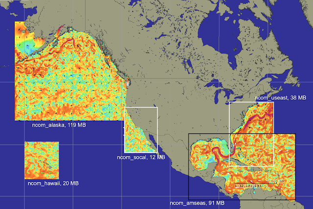
What I want to stress here is, that for work on land, or more specifically, when you have an internet connection available, anyone can easily get this NCOM data for planning or analysis, and it will display nicely in any of the popular navigation and weather programs, such as OpenCPN or qtVlm, as well as other popular commercial programs such as Coastal Explorer or TimeZero. Luckily, the data are subdivided into several regions, but even so, these regional files are too large to load by sat phone or cell phone at sea... with maybe the exception of 4G or 5G service in coastal waters, which is evolving technology.  

Available data sets are shown in the picture below.


NCOM data sets loaded into qtVlm. The region called "Alaska" could be called "NE Pacific."

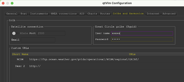
The files are located at this link

https://ftp.ocean.weather.gov/grids/operational/NCOM/regional/GRIB2


You can download them directly from that site, which includes the last several model runs; we would typically want  the most recent. If you are using qtVlm you can identify this URL as a "Custom grib" source and then access the files directly within the program, which loads them as well. As an example of such an interface, that set up page is shown below


Then when ready to load the grib into one of three slots, we select the Custom Grib tab and see this:


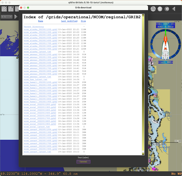
Click the file and the data loads into the program. If you have not viewed currents before in your nav program, you may need to go to the grib display set up to select display options.

Besides the value for ocean routing, an intriguing possibility is to use these data to supplement routing on inland waters where currents, primarily tidal, can have such a large effect. Below is an example of the NCOM forecasts reaching into the Strait of Juan de Fuca viewed in LuckGrib.

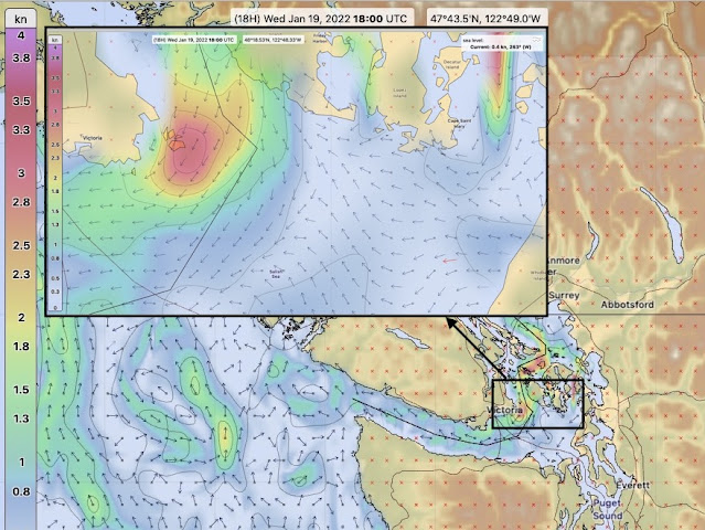
There is a lot of detail forecasted in this model, much of which we can actually check. 

Here are a couple more examples from the Rhode Island Sound area, this time looking at the data in qtVlm. 

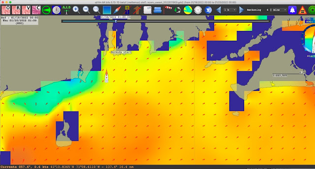
There is not a color bar scale. The values at the cursor show up in the status bar. But roughly, medium orange is 0.6 or 0.7 kts; darkest orange is 1 kt; yellow is 0.3 or 0.4 ; green-blue is 0.2, 0.1.

Comparing this to NOAA tidal current predictions is not very fruitful, but that should not be discouraging. It can be done, but it is difficult, primarily because the tidal current predictions are given as reversing, whereas in this open water they are largely rotating. Thus reading carefully you see NOAA tells us only the "average" of the flood and ebb directions. If you look at any one specific time, you are likely not seeing water flowing in the "average direction."

We do better using HF radar measurements of the currents, which you will find also do not agree with the NOAA tidal current predictions, but they do offer encouraging support for the NCOM forecasts. A sample is below for the time of the above data.


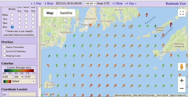
Here there is a color bar, and I think it is fair to say that this is about all the level of accuracy we should impose on these measurements. We can click each picture for precise read outs, but that might be over doing the actual accuracy.  All and all, the general flow and rough speeds are about right.  We do not really need more than that... but it would be nice to see a case where the flow is notably different, and that is shown below.

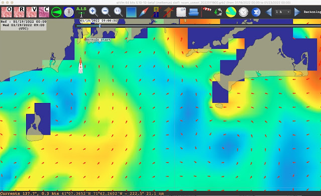
This is a view of the area 16 hours earlier. The speed color code is the same as above, and the range in speeds is about the same, but the flow is notably different, with a clear eddy below Martha's Vineyard. The HF radar measurements at this time are shown below.

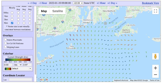
We see here a very nice confirmation of the forecast. The eddy shows up in about the right place and the other changes in flow pattern from above are reproduced.

These are just two ad hoc checks done here at random at the time of writing, but they look promising and hopefully with these notes more navigators will look into this resource and test it various ways.  It seems logical for coastal ocean routing, but we have a lot of work to do to learn of its value for more inland sailing. 

Thursday, January 13, 2022

Collision Avoidance Using AIS

Most navigation programs (electronic charting systems, ECS) will read and display AIS targets provided to them by a live AIS receiver on the boat or via an internet connection. The former source is much preferred because the internet sources are notably delayed; internet AIS can be very useful for training, but underway it is mostly for a general awareness of who might be in the neighborhood, not where they are at the moment and it cannot be relied upon for collision avoidance.

Most of the ECS AIS displays also show the age of the individual reports in seconds that can be compared with the standards shown below, which is adapted from our post Introduction to AIS.  This makes it clear to the user that they are being updated as required.


A typical display of AIS traffic is shown below. In this ECS (qtVlm) there are several options for learning about a target and also our interactions with it, which is the subject at hand that we get to shortly.


The dark blue reports are tooltips. Only one at a time would show and then disappear when the cursor moves. The CPA info in white background can  be turned on for any vessel. Ours is the white one in center screen. The Details can be turned on for one or multiple targets.  It is not the subject at hand, but the voyage data sent out may not be right. Here we see a vessel reported as "moored" that is moving at 12.7 kts, and another marked as engaged in fishing, which in fact will not be fishing till it gets back to Dutch Harbor. We can't blame the ECS for marking it with a fishing daymark, because that is what it was told.  Again our reminder: To see details, click the pic, then right click and open in new tab, and then zoom.

In the above picture we do not have the collision avoidance functions turned on. We are seeing the COG predictor lines set for 6 min. The end of the green dashed lines is where the vessels will be 6 minutes from now.  It is usually best to have this reckoning time be the same for our vessel as it is for the target vessels. This much is already very valuable information, but in fact the ECS can do much more than that.

Short of using those computed collision avoidance displays, that is what we have to work with, the COG predictor lines of our vessel and the targets, and the goal at hand here is see what can we learn from just these predictor lines.  

For any discussion of collision avoidance we must return to the Navigation Rules that tell us about collision risk in Rule 7, and in particular Part (d) (i)

Rule 7 - Risk of Collision
(a) Every vessel shall use all available means appropriate to the prevailing circumstances and conditions to determine if risk of collision exists. If there is any doubt such risk shall be deemed to exist.

(b) Proper use shall be made of radar equipment if fitted and operational, including long-range scanning to obtain early warning of risk of collision and radar plotting or equivalent systematic observation of detected objects.

(c) Assumptions shall not be made on the basis of scanty information, especially scanty radar information.

(d) In determining if risk of collision exists the following considerations shall be among those taken into account:

(i) Such risk shall be deemed to exist if the compass bearing of an approaching vessel does not appreciably change.

(ii) Such risk may sometimes exist even when an appreciable bearing change is evident, particularly when approaching a very large vessel or a tow or when approaching a vessel at close range.


First, modern court cases have established that "all available means" definitely includes ECDIS (for commercial vessels) or ECS for those without ECDIS, and that AIS is now on par with the radar requirements.  In short, these are powerful tools and it is essentially negligent not to use them if available.

For present considerations, the key point is (d) (i), which tells us how to detect risk of collision using compass bearings. Note the word "shall"; this is not a suggestion, nor an option, it is required.  In basic navigation we often teach a shortcut using relative angles on the bow.

The above is from our textbook Inland and Coastal Navigation. This method assumes the heading of our boat does not change during the observation. Using actual compass bearings removes that uncertainty.

We can apply this principle to the display of AIS projectors, because we have in effect two views of the target taken 6 minutes apart, or 12 minutes if we used that. If the bearing does not change we are on a collision course. If the bearing moves toward the bow, the target is crossing in front of us; if it moves aft, we are crossing in front of it, as illustrated below.


Below is a compilation to show that the concept of bearing moving toward or away from the bow can be applied to targets seen in any direction.


So even without sophisticated closest point of approach (CPA) functions, we can determine if a target is crossing in front of or behind us... that is, as soon as we are able to measure or estimate the bearing to the target from preset positions and also from the tips of the projection lines which would be the bearings we see after watching the target for 6 min or 12 min.  Six minutes is a popular reckoning choice, because at 6 min the length of the predictor line (nmi) is one tenth of the boat speed  (kts).  At 12 min prediction, we divide the length by 2 to get the speed.

Most ECS display the range and bearing to each target, so we do not have to measure the first one, just read it.  Also all ECS  have a quick measurement tool or ruler tool that we can use to measure the bearing from our projector tip to the target projector tip, and that is then the second bearing. Below is a sample from qtVlm. We are left then to reason through the direction we are looking and decide if this is toward or away from the bow.... or if we are on a collision course. 

Keep in mind that a collision course is indeed a rare thing. Just a degree or so (that we cannot really measure in this method) will bypass a collision, and a notable degree change is a fairly big separation.


Here the red lines and dashed magenta line were just added for perspective. We read first bearing from the tooltip and then use ruler tool to learn that the next bearing would be notably forward so this target is passing in front of us.

If we then turned on the closest point of approach (CPA) data we would see this immediately. Below is that view about when they cross.


We see that indeed this target passes well in front of us, and we will have CPA in 8 min, and the CPA will  be 1.1 nmi. Notice where our 6 min position is compared to 2 min later at CPA.  With this type of data we can get these forecasts from a long distance off, but that brings us back to Rule 7 (c), which is the good advice for radar observations that also apply to AIS computations. We do not want to rely on such data from a long ways off, where just slight course changes or current sets can affect the later CPA. 

Note that the AIS gives us both COG and true heading for those vessels with a heading sensor, so we can often get an idea about the currents—and maybe understand why their tracks are drifting off to one side of the traffic lanes or other obvious fairway routes.  We saw this very nicely in our reenactment of the grounding of the Ever Given in the Suez Canal.


I will add more examples later on, with and without the CPA info to illustrate this point.

To keep this in perspective, our logical first choice is to learn how to use the CPA configurations in our ECS and these then typically solve the problem of collision risk evaluation. But if you are new to an ECS on a new boat, you may not know or understand what is being shown, so this basic view of the targets based on COG predictors alone could be helpful. Also sometimes the CPA configuration for AIS can have multiple settings to account for various conditions, which means there is the chance that they are not set up in the optimum manner for present conditions.

Also, needless to say, learning whether a target is crossing in front of you or behind you is just the beginning of our obligation in the Navigation Rules.  From Rule 7 we move on to Rule 8, Action to Avoid Collision.


Saturday, January 1, 2022

Compare Pub 249 and Pub 229 Using the Celestial Tools App

Celestial navigation sight reduction when done manually these days is primarily with the aid of Pub 249 or Pub 229. The former was developed for aviation; it is somewhat easier to use than Pub 229, the marine navigation standard, but is less precise in that air navigation by cel nav is less accurate to begin with because of the speed of the aircraft.

Nevertheless, Pub 249 remains popular with many ocean sailors. All USCG exams, on the other hand, must be solved using Pub 229.

Pub 249 rounds calculated heights (Hc) to the nearest whole arc minute, making them effectively ± 0.5' in precision, with azimuths (Zn) given to the whole degree, meaning ± 0.5º, whereas Pub 229 gives the tabulated values of Hc to the nearest 0.1' and azimuths to nearest 0.1º.  This does not, however, tell us how much a position fix might vary using these two different solutions. There are too many variables involved in that we have to look at the intersections of plotted lines of position that can be in more or less random directions.

We can look into this difference using an extensive practice exercise on running fixes (Exercise 6.6) from our textbook Celestial Navigation, which we can solve using a unique function of the free PC software app called Celestial Tools written by the late Stan Klein, an innovative and dedicated navigation instructor. Stan originally developed this tool for Power Squadron (USPS) members and instructors, and then made it available to the public. We have hosted his latest versions of the app for many years, and continue to so so, as was his wish.


There are 5 more exercises like this one in the textbook, each yielding practice with 3 running fixes (1 to 2, 2 to 3, and 1 to 3).  They cover all hemispheres and various course headings.


This is the graphic index from Celestial Tools. The function we are using is "SR Methods & Fix," which is a tool that tells us each of the intermediate answers to a sight reduction process for the various tables available plus the direction computation.  There is a description of the  all of Celestial Tools functions that supplements the included Help file. Find all of these in the Starpath Downloads page.

This exercise offers three running fixes we can use to check the differences between using 229 and 249. It is a unique form of exercise, copied from USCG license exams, which I will come back to. All sextant corrections are done; all Nautical Almanac lookup is done, so we are left to using the sight reduction tables to find Hc and Zn and then plotting two or more of the LOPs and advancing them to the same time for a running fix.

Below are the the data screens from the SR Methods & Fix function using 249 and 229 for the 1015  sight.

The first step is updating the DR to the times of the sights starting from the given position at 0900 WT. These results are shown below.


1015 sight reduced with Pub 249


From Pub 249 we get Hc = 58º 53' with a = 17' T 099º (which rounds the measured Ho minutes of 9.7' to to 10' according to 249 instructions, but we have no real reason to do that). A better result is Pub 249:  a = 16.7' T 099.

A short digression about the bottom center output show: The USPS and the Coast Guard Auxiliary define what they call an estimated position as the nearest point on an LOP to the DR position. That accounts for what you see here in this output labeled EP. This concept, however, has no real practical value for ocean navigation under sail, which is our main student body. Hence we not only do not teach this, we strongly discourage its use. It is much more likely to be misleading than to be helpful.

The best way to determine an "estimated position" is to use the log and compass DR corrected for everything you know of that might shift that position. In our terminology, we do not distinguish a DR position from an estimated position. This is the historical definition of a DR position that we adhere to. Certainly the best EP will indeed be located someone on the latest LOP if you have one. That is a definition of the LOP, but the nearest point on the LOP to the corresponding DR is not inherently anything more than uninformed wishful thinking.


1015 sight reduced with Pub 229

From Pub 229 we get Hc = 58º 53.6' with Pub 229: a = 16.1' T 097.6º  (Stan chose to round this to 098, but we do not need to do that. With care, we can plot to fractions of a degree.)

This example finds the a-values differing by 0.6' and Zn differing by 1.4º between 249 and 229.

Now we look at the 1156 sight.

1156 sight reduced with Pub 249

From Pub 249 at 1156 we get Hc = 80º 16' with a = 22' T 139º.

1156 sight reduced with Pub 229

From Pub 229 at 1156 we get Hc = 80º 16.4' with a = 21.6' T 135.8º.

Now we carry out a running fix between 1015 and 1156 sights using both reduction methods. We will compute this plotting as we are looking for small differences, but it could be done by hand.

From Pub 249
for the 1015 sight we have: AP 22 N, 124º 47.1' W,  with a = 16.7' T 099º
for the 1156 sight we have: AP 22 N, 125º 4.1' W,  with a = 22' T 139º

With speed 13.0 kts on course 250, we have a run time of 1h 41m and a distance run of 21.9 nmi.

From Pub 229
for the 1015 sight we have: AP 22 N, 124º 47.1' W,  with a = 16.1' T 097.6º
for the 1156 sight we have: AP 22 N, 125º 4.1' W,  with a = 21.6' T 135.8º

From the computed intersections below, we find that the pub 249 fix at 1156 is  21º 39.6' N,  124º 53.2' W and the Pub 229 fix is at  21º 39.3' N,  124º 53.7' W.  

Note the special convention on angle formats in this calculator.

Rfix 1 to 2 using Pub 249,


Rfix plot 1 to 2 using Pub 229.


These two positions are just 0.55 nmi apart, which is quite a surprise in that the 1156 Zns differ so much (139 vs 135.8).


________________________

We can now do the third sight reduction at 1425 and get another rfix from 2 to 3.

1425 sight reduced with Pub 229

From Pub 229 we get Hc = 60º 42.6' with Pub 229: a = 12.3' T 261.1º  (Again, we do not need to round Z when figuring Zn.)


1425 sight reduced with Pub 249.

From Pub 249 we get Hc = 60º 42' with Pub 249: a = 12.9' T 259º 

This example finds the a-values differing again by 0.6' (a coincidence) and the Zn differing by 2.1º.  For the rfix from 2 to 3 at 1425 we have:

From Pub 249
for the 1156 sight we have: AP 22 N, 125º 4.1' W,  with a = 22' T 139º
for the 1425 sight we have: AP 22 N, 125º 18.1' W,  with a = 12.9' T 259º

From Pub 229
for the 1156 sight we have: AP 22 N, 125º 4.1' W,  with a = 21.6' T 135.8º
for the 1425 sight we have: AP 22 N, 125º 18.1' W,  with a = 12.3' T 261.1º

From the computed intersections below we get for the pub 249 fix at 1425 of  20º 47.4' N,  125º 17.0' W and for the Pub 229 fix: 20º 41.5' N,  125º 18.3' W  


 Rfix 2 to 3 using Pub 249

Rfix 2 to 3 using Pub 229

These two solutions differ by 6 nmi, which is quite different from the sight 1 to sight 2 offset between sight reduction tables. 

We begin to see the issue involved. In the first case the sight reduction differences were larger than in the second case, but the second case had 10 times larger offset in final positions. The first difference was frankly smaller than I would have guessed, and the second one was larger than expected. Keep in mind that the 229 solution is the better one, and we are seeing here the cost of the lower precision of 249. These differences are mostly due to the Zn values and we can improve on the 249 values with interpolation, as outlined below.

____________

We can do one final test with a running fix from sight 1 to sight 3, and for these we have the solutions already done.

From Pub 249
for the 1015 sight we have: AP 22 N, 124º 47.1' W,  with a = 16.7' T 099º
for the 1425 sight we have: AP 22 N, 125º 18.1' W,  with a = 12.9' T 259º

With speed 13.0 kts on course 250, we have a run time of 4h 10m and a distance run of 54.2 nmi.

From Pub 229
for the 1015 sight we have: AP 22 N, 124º 47.1' W,  with a = 16.1' T 097.6º
for the 1425 sight we have: AP 22 N, 125º 18.1' W,  with a = 12.3' T 261.1º

The pub 249 fix at 1425  is at  21º 29.3' N,  125º 25.8' W

The pub 229 fix at 1425 is at  21º 28.9' N,  125º 26.3' W  


We then compute the distance between these two:


And we see that they differ by just 0.6 nmi, which is similar to what we saw in the sight 1 to sight 2 rfix. In this case we can also compare the fixes we got from 1 to 3 with what we got from 2 to 3.

In principle the 2 to 3 would be the better fix in that it is a shorter run so the errors in the DR are less crucial, and also the 1 to 3 sights let the sun get too far west so the intersection angles are not as good: 2 to 3 intersection at 54.7º and 1 to 3 at 16.5º.

2 to 3
Pub 249 fix at 1425  is at 20º 47.4' N,  125º 17.0' W 
Pub 229 fix at 1425  is at 20º 41.5' N,  125º 18.3' W  

1 to 3
The pub 249 fix at 1425 is at  21º 29.3' N,  125º 25.8' W

The pub 229 fix at 1425 is at  21º 28.9' N,  125º 26.3' W  


It is left as an exercise for those who want to study this more to work through the remaining examples using this procedure.

One way to improve the values of Z for any tables we use is to interpolate Z for the declination minutes. The standard procedure with 249 or 229 always takes Z from the degrees part of the declination, which was 14º in these examples. In all cases, however, the dec minutes were very large, so we would have gotten better results by using 15º dec to find the Z value. In this example it would have got 97 for 249 and 97.4 for 229, making the final fixes a bit closer still.