Thursday, January 31, 2013

State of the Art Ocean Current Presentation

RTOFS ocean currents predictions are shown here updated daily centered on the near realtime (updated every 2h) location of a vessel underway.  The currents are computed daily at 14z, with initialization time of 00z, with 144 hourly predictions. We show here the data every 6h for 3 days.  

Speed changes at whole knots are marked by a contour line.

The vessel being followed in this example is the rowboat James Robert Hansen (www.oarnorthwest.com) on a 3,600-nmi voyage from Dakar, Senegal to Miami, FL.

There are three vessel positions shown: the latest position, the position 24 hr earlier, and the historic or projected position at the time of the forecast. To see the predicted currents at the present vessel location,  scroll down until the two leading positions overlap.  Also shown are the course made good and speed made good over the past 24 hr.

To view the trends, just click open any one picture, then scroll (mouse roll) though the set to implement an animation of the pattern.

We have an overview of ocean currents at www.starpath.com/currents. These data are from the Hi-res Atlantic RTOFS model.

This presentation and the implementation of it is the fine work of Angeline Pendergrass of the UW Atmospheric Sciences Department. She is the coordinator of the weather forecasting team for this expedition.

00z Today
06z Today
12z Today
18z Today
00z Tomorrow
06z Tomorrow
12z Tomorrow
18z Tomorrow
00z Day after Tomorrow
06z Day after Tomorrow
12z Day after Tomorrow
18z Day after Tomorrow
00z Three days out


Sunday, January 20, 2013

UTC by Lunar Altitudes (Celestial Navigation)


This is a way you can find UTC underway if you have lost it using only standard methods of sight reduction. This article solves the problem using a calculator solution, but this can also be worked by traditional tables and plotting with an expanded scale. The calculator used here was an early version of the StarPilot, which was developed at Starpath.

This method is often called GMT by "Lunar altitudes" as opposed to GMT by "Lunar distances." To our knowledge, the first person to describe the lunar altitude technique in modern times was John Letcher, author of a wonderful, though sadly obscure celestial nav book called Celestial Navigation with HO 208, but he is more famous for his also pioneering work on self-steering equipment. Sometime later, but independently, the technique was also described by Francis Chichester. Chances are if we look back into the last 100 years or so of of textbooks on cel nav we would find that someone else had also proposed something like this, in some form. The principle was known hundreds of years ago.

The better known Lunar Distances method is more generally applicable but it requires special sights and special analysis. The Lunar Altitudes method can be done with normal sights and normal procedures.


This post is also an experiment in digging out of the recesses of our website old articles and making them more readily available. Thus this is text from about the year 2000.

* * *

 The prerequisite for the technique is a moon bearing near due east or due west at twilight. We also assume we have a watch that is running properly, but it has an unknown error in it. Our task is to use celestial measurements to determine the watch error of this watch — it can be minutes, hours, or days, but let's assume we know the day. (We have an article on how to do this we will post later.)

The simple principle of this technique is this: if we take 3 simultaneous sights, 1 each of two bodies that intersect in a good angle for a fix, and a third sight of a moon lying near due east or west, then the longitude difference between the 2-body fix and the moon's LOP is a measure of our watch error. In other words, if the watch were exactly right and we took 3 precise sights, then all 3 lines would intersect in the same place which was our true position. If the watch is wrong, the moon line will defer from the intersection of the other two, and the amount it is off is related to the watch error. Note that the latitude of the 2-body fix will be our correct latitude, even though the watch time was in error.

Example:
We have other examples of this technique worked out in our study materials and there is also one in our Emergency Navigation Book, but driving home tonight at twilight headed due east, almost straight toward a beautiful full moon, it was compelling to add a new one for users of our new StarPilot calculator. The date is Jan 19, 2000. The time is 1750 PST (ZD = +8) — but we suspect there is some error in this watch time (surprise, surprise!). Planets, stars, and a beautiful full moon fill the sky. Our DR position (also uncertain as it must be, if this is to be any challenge at all) is 47° 45' N, 123° 05'W. Our job is to figure out what the watch error is.

For this example, we will also assume that you have read through the other parts of the StarPilot description so you know more or less how it works... in other words, we will not review all the input steps here.

After taking the 6 sights listed at the end of this exercise, we plot out the results to establish what we would have obtained had we taken all 3 sights simultaneously. Naturally this cannot be done simultaneously, but if we take the series of sights 1-2-3 then 1-2-3 again, we can graph the results and interpolate a set of simultaneous values. This is a normal technique often done at sea to minimize running fix corrections. We take the moon, and two nice bright planets.

ZD=+8, WE = ? (but enter as 0 sec), HE = 9ft, IC = 0, DR = 47° 45' N, 123° 05'W, date = Jan 19, 2000, our speed = 0.


WT         body      Hs          LOP
17:50:00   Mars      25° 04.9'   a = 18.2' T 223.5°

17:50:00   Moon      19° 30.2'   a = 18.7' A 081.5°

17:50:00   Saturn    52° 37.5'   a = 03.5' A 154.6°


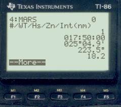
Note that the moon was indeed about due east, off only 8.5°.


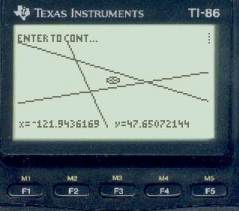
After the 3 sight reductions, we do Fix by plotting option with Speed = 0, and get the picture on the right. We will clearly have to zoom in on this to see what is going on in detail, but some things are already apparent. Our DR is far off to the east (circle in the center with the cursor in it), and we can tell already that we have a watch error — the near vertical moon line does not go through the planet fix. We also know — or you will know after you practice this some — that our watch is fast since the moon line lies to the east of the planet fix. And from the planet fix we can see that our DR lat is also too high. Remember, the lat of that intersection is correct, even though the longitude of it is clearly not correct. 
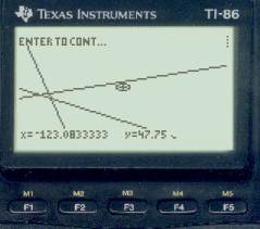
Now we start to zoom in by moving the cursor to the center of the LOPs as shown below top left and then press Enter and update the DR to that position and replot with a scale of 3 to get the picture next to it.


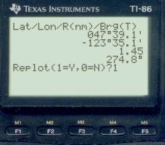
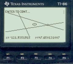
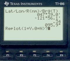
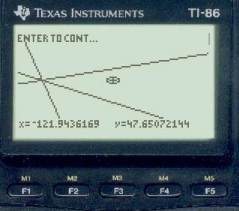
We need to know now how far east the moon line is of the planet fix, so set the cursor on the planet fix (below left) and press Enter to get the Lat-Lon of that location (bottom right). From this we see that our proper latitude is 47° 39.1 N and the longitude of this intersection is 123° 35.1' W (not our correct longitude yet since we don't know the time yet).


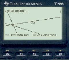
Now move the cursor to the moon line (below left) at the same Lat and press Enter to get that data as shown below right.


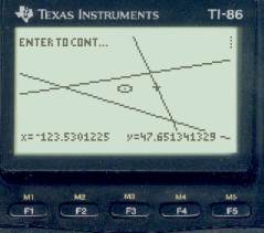
This longitude is 123° 31.8' W, which is 3.3' east of the planet fix. Our next step is to guess from this how much the watch is fast and then adjust it by that amount and do the sight reductions again. Each time we do an iteration like that we should get closer, and when all 3 lines coincide we can assume we have the right time.

Note the obvious, however, that we are assuming all sights are precisely accurate. Even a small sight error will cause a relatively large time error. And the analysis here is a bit more complicated than normal time evaluation. For example, if we do a 3-star fix that makes a nice tight triangle but unknown to us our time if off by 1 minute, the lat will be right, but the longitude will be off by 15' -- too far west if the watch is fast, and too far east if the watch is slow. But this analysis does not help us find our watch error from the moon sight.

Here we must consider that the moon is moving relative to the stars at the rate of about 360° every 30 days or 12°/day or 12x60'/24x60 min = 1'per 2 min of time. So our 3.3' discrepancy would correspond to a time error of about 6.6 minutes. Hence our first guess is that we are 6m 36s fast.
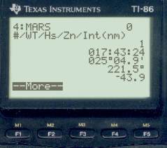
Now we redo the sight reductions at the new time of 17:50:00 - 00:06:36 = 17:43:24 WT on Jan 19, 2000. Note our DR has been stored in roughly the middle of the lines (47.39, -13.329) but it does not matter where this is for the sight reductions.

WT         body      Hs          LOP
17:43:24   Mars      25° 04.9'   a = 43.9' A 221.5°

17:43:24   Moon      19° 30.2'   a = 63.8' T 080.1°

17:43:24   Saturn    52° 37.5'   a = 30.1' T 151.3°


Then do fix by plot to get the screen on the right, below.


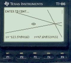
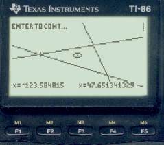
We are definitely closer on the GMT, but will need to rescale the plot to go on. Move the cursor to the center of the LOPs, update DR, and replot (left below). Then move cursor to center again, update DR and plot with scale of 6 to get right side below.


Our time correction was clearly too big, we have overshot the mark. Now lets see how many minutes too far we have gone. As before, set cursor on the fix and read the longitude, and then set cursor on the moon line at the same latitude to read it.


The difference is 0.9', or using our previous estimate, 0.9 x 2 = 1.8 min = 1m 48s. This would imply that our time error was not 6m 36s fast, but 6m 36s - 1m 48s = 4m 48s fast. BUT, we know from the first iteration that 2m per 1' is too big a rate. We wanted to move 3.3 and we moved 3.3 + 0.9 = 4.2. In other words, we should reduce our rate by 3.3/4.2 = 0.79. So, 1.8m x 0.79 = 1.4m = 1m 24s, and our better guess is 6m 36s - 1m 24s = 5m 12s.

So once again, redo the sights with a new time: 17:50:00 - 00:05:12 = 17:44:48.
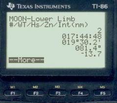
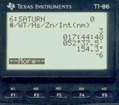
WT         body      Hs          LOP
17:44:48   Mars      25° 04.9'   a = 09.5' T 223.4°

17:44:48   Moon      19° 30.2'   a = 13.7' A 081.4°

17:44:48   Saturn    52° 37.5'   a = 06.0' A 154.3°


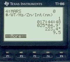
Now, again, move the cursor to the center of the fix, update DR, and replot with a scale of 10.


Now we are essentially done, the fix is very good now — note from the right-side screen that the range DR to fix is 1.78 miles, so this is a very tight triangle and we have found that our watch error was 5m 12s fast.

The true error was 5m exactly, so this turned out well. The main constraint on this method is it requires a moon lying near east or west at twilight. This one off by 9° worked fine. Practice with various conditions to see what the limits are. The virtue of this method is it takes only standard sights, no special sextant handling and no special computations. We just iterate the time till we get the lines to coincide.

Saturday, January 12, 2013

A Real OMG Omega Block over the E. Pacific

When the winds aloft form into the shape of the Greek letter Omega (Ω), they tend to resist changes both aloft and on the surface. This is the type of pattern mariners like to see as we then have more confidence that things tomorrow will be much like they are today. This tends to me more useful in the summer than winter, because we are not likely to be in the North Pacific in the winter... unless of course we have a job that forces us to be there. And in the winter there is much more activity to disrupt the pattern.

Here is what we see today, which is a rather remarkable example of such a pattern. These are the winds at the 500 mb level, at about 18,000 ft.


Here is the huge blocking High below it on the surface."Blocking" in the sense we use in our classes, meaning [1] more or less in the right place (ie due west of San Francisco, on the rhumbline from WA to HI), [2] central pressure higher than 1030 mb, and [3] with at least 2 nearly round isobars encircling it.


Here is the surface 48 hr later, and we still see more or less similar High pressure, but this is the winter, so look at the real butt kicking Low coming at this pattern. It cannot withstand that sort of attack too long.

 Even with this, 96 hr later we still have high pressure dominating the Eastern Pacific


And 96 hr later the omega block starts to give in to the attacks from the west. At this point, we no longer have any idea what the surface will look like the next day.... until the NWS tells us, and even in this case we will have to use all forecasts with caution because it seems a cut off low is in the process of forming which usually means the surface forecasts are more in question. 


Thanks to Starpath instructor Larry Brandt for alerting us to this notable example taking place.

Tuesday, January 8, 2013

Ocean Currents

Here is the picture of ocean currents as we study them in many navigation textbooks:


RSMAS at University of Miami is a good place to get an overview of the various current systems. (If you use their excellent resource, please help support them by signing their Guest Book. It is a link at the bottom of the home page index.)

Here, on the other hand, is what the ocean really looks like. In other words, there are average flow patterns as seen above and these have names, Gulf Stream, Equatorial Counter Current, etc, but at any one moment, at any location, you might experience one of these eddies or meanders that are spread across the ocean, in which case you could experience quite different currents than any climatic prediction for where you are. Pilot charts are one good way to get climatic predictions for specific locations and times, worldwide. (It is hi-res. Go to full screen.)


We learn much about these currents these days from satellite images and from ocean models. Below is another remarkable video from NASA that shows some element of the actual current speeds in these eddies. You can assume the color code for speeds is about what we showed in an earlier post, namely the red marks speeds of 5 kts or so, yellow-green around 4 - 3 kts and the turquoise is 2 - 1 kts. In short, these are strong currents to a small boat at sea.


In either of the above movies you see the famous Gulf Stream current (complex as it is) running up the east coast of the US. (The counter part in the Western Pacific along the coast of Asia is called the Kuroshiro current.) This current system is the best known and documented of all, but we are still learning much about it from new resources. Below is Benjamin Franklin's map of the Stream from 1770.

Our immediate interest in ocean currents is to assist in routing of the OARNW row across the tropical Atlantic with the hopes of getting some actual measurements of anomalous eddies along the way.  See Row Boats in Ocean Currents.

For another look at our dynamic ocean, see this Navy animation covering Gulf of Mexico and Caribbean.  Note from the dates shown how long some of these eddies and loops can persist, and how the loops can pinch off into eddies. This type of behavior has been well known to mariners for the northern Gulf Stream for many years, but we see now that this occurs many places in the oceans.


The second goal is to update our training materials on new resources for predicting ocean currents underway, which starts with recognizing that it is not as simple as once thought. We are fortunate to have some very powerful new resources.

As an example of using these data for navigation planning, look at this 144h forecast for the Atlantic and notice the small transient eddy off the coast of Dakar, western most tip of Africa at about 15N.


Here now is the type of data we can provide the boat on a daily basis to plan their navigation. This is that Dakar region, before reaching the Cape Verdes.  This is RTOFS data from NCEP.

and
In other words had they left a couple days ago they would have hit a huge flush to the south which is not what they want.  The (NE) trades have a strong northerly component in them till well past the Cape Verdes so they have to be careful not to get pushed too far south earth in the crossing or it will be hard to maintain course in the NE wind across the ocean.

_____________

Note added Apr 27, 2013:  we have set up a more general link to current resources at www.starpath.com/currents.


Thursday, January 3, 2013

It is Raining – What does that mean? Part 3

More on rain... will it never end?

Below is a snapshot of global rainfall from the NASA.


Recall, I am trying to understand rain rates so we can interpret what we see when it rains. There are two earlier articles:

Part 1 Covers definitions and background 

Part 2 Gives an example of rain at the border between Light Rain and Moderate Rain


I think we see from any of these NASA videos that most rain by area worldwide is Light Rain, meaning below 0.10"/hr, and most of the world's rain falls into the oceans. This is not just because there is more ocean than land, but it clearly shows that their are more rain clouds over the water than over the land. This probably makes sense from some basic hydrological reasoning.

You may find it interesting to note that rain fall rates are often presented on a logarithmic scale, meaning the range we can detect and be subject to varies my orders of magnitudes — not factors of 2 or 3, but factors of 10 or 100. We have (in inches/hr)

Drizzle = 0 to 0.04
Light Rain = 0 to 0.10  (There can be distinctions between low level light rain and drizzle)
Moderate Rain = 0.11 to 0.30
Heavy Rain = 0.31 to 2.0
Violent Rain = > 2.0  (This is new a category not mentioned till now in this series, discussed more below))

A short diversion on rain gauges

The smallest unit of rain fall that is commonly measured is 0.01" corresponding to one tip of a tipping bucket rain gauge. For those who have not thought of such matters ( I was in that category not long ago ) here is a short crude demo of how they work.  I am not at all sure what their accuracy is. We will check that later. This was an inexpensive unit, but it seems that there is some factory in China making all of them, so I would guess they have homed in on the dimensions and engineering pretty well. I have just ordered another one online, looks the same as this one, wireless, for $32 including shipping.  We shall see.  An expensive US model that sells for $500 promises 2% up to 1"/hr and 3% up to 2"/hr.  The latter (2"/hr) is the defining point for Violent Rain, the next and last category after Heavy Rain. As you see below this is a pretty simple device.

This one has a cone collector with diameter of 4.41 inches (112 mm). Thus a cylinder of water 0.01" tall on it would include 0.153 inches cubed of water (pi x r^2 x h), which is 2.50 cc, which turns out to be about 0.5 teaspoons. Thus each half teaspoon of collected water should give a tip, as indeed it does.


PS. At the end of the video it looks like I knocked the bucket over with the teaspoon to make my point, but that is not the case. It honestly tipped at the right time, to the drop!  All crude stuff, but it does show how it works and that it works about right.

Get 1 click in an hour (0.01") and you have barely measurable drizzle.  Get 10 clicks in an hour and you have 0.10"/hr which is the top of Light Rain or the bottom of Moderate Rain. The assumption might be that if you did get 10 clicks per hour with the onset of a new steady rain that these would be 10 more or less evenly spaced clicks, namely 60 min/10 clicks, or one click every 6 min or so.

But now we run up against the programming limits of an inexpensive device. As far as i can tell from the LaCrosse instrument, it is just accumulating the clicks and not computing an hourly rate based on what it knows.  That is, in principle, after the second click 6 min later, it might guess that the actual hourly rate is 0.10"/hr, even though it has only collected two clicks over a 6-min period, but that is not the way this one works.  It just counts the clicks and even looking out the window to see this is indeed a steady rain fall, your gauge will show a building rain rate for the first hour.  So you do not really know what the hourly rate is from the read out alone until it has collected rain for an hour or more.

If you were really-really into this, you could time the clicks yourself and compute the rate before the hour.  In fact, even with a cheap one like this you can download the data and deduce the rate after about 15 min or so.  I still have no idea how accurate that would be.

I suspect that a higher quality instrument would do this differently.  In other words, there are some rain gauges alone that cost 500 to 800$, so these would presumably be more accurate in their tips and also have software that actually computes a live hourly rate based on the actual time rate it collects rain.  These instruments would then show a dynamic hourly rate based on fluctuations in the actual rate.

To follow up on this we have purchased an even cheaper rain gauge from Timexweather. It was $32 including shipping on amazon.  Next we will test this one and report. I know the tension must be building.


Violent Rain

The last thought to add to this note is the concept of a rain intensity called Violent Rain, which is >2"/hr. Now this is indeed violent, but nowhere near world records which are above 10"/hr for short periods.

The NWS does not use Violent Rain scale and it is not in their Forecasting Handbook No. 1 as a classification for observations. They go up only to Heavy. The term is in use by the UK MetOffice, which you will note also calls Light Rain = Slight Rain. Recall the NWS has this mixed up in the Handbook, using both phrases for the same intensity.

I believe there is a value to the term Violent Rain, even though any level of Heavy Rain is really heavy, because mariners who might sail in squalls, especially those on the fringes of a hurricane will definitely see Violent Rain. I have seen this a couple times, once very dramatically. It was in a tropical system near HI, and in one squall we were standing in the cockpit of a 40-ft boat and without exaggeration we could not see the bow! It was like standing under a faucet. We were dumb struck as we stood there laughing at such an amazing demonstration of nature.

The other interesting aspect of this observation was we were in 30+ kts of wind, and this rain had totally beaten down the waves till they were a smooth rolling sea of swells only.

If you do a Google Search on "violent rain" you will see that this term has worked its way into our subculture to a high degree. It is used to name a huge range of endeavors.  I am sure, however, that those who use it, do not appreciate the actual nature of their namesake. They just have a feeling that it must be significant.  They are right.

Living in Seattle i do not think we will ever get a sample of this rain intensity to show here, but we are in daily contact with several boats in the tropics, and we will ask them to be sure to make a video if they run across it.  We will ask our friends at OARNW to watch for this as they spend some 60+ days rowing across the tropical Atlantic from Dakar to Miami.