Friday, December 31, 2021

True Wind and Ground Wind—and Why We Need Both

When we are underway, we measure the apparent wind speed (AWS) with an anemometer and the apparent wind angle (AWA) relative to the bow with a wind vane. We also read the course through the water (CTW) with a heading sensor and the speed through the water (STW) with the knotmeter. Thus we can find the apparent wind direction (AWD) from AWD = CTW+AWA, and from this we can solve for the true wind speed (TWS) and true wind direction (TWD), as shown below. 

This true wind, shown on the left above, is what sailors care about—more specifically, what the helmsman and trimmers care about, because this is the wind their target speeds are tied to as presented in the polar diagrams.

The navigator and tactician, on the other hand, have the job of planning the route ahead, so they need to know if the wind we are experiencing now is what the forecasts said it will be, and they need to know if the changes in the wind that have taken place are consistent with the forecasts. To do this, they cannot use the same "true wind" that the trimmers use, unless the (COG and SOG) vector is the same as the (CTW and STW) vector. These two vectors can differ for a lot of reasons, including instrument calibration and steering bias, but the usual cause in a well founded vessel is actual motion of the water, currents.

The wind in the forecasts is "ground wind," meaning it is relative to the fixed earth, the ground. The true wind on the left above is relative to the water, and if that water is moving the ground wind will not be the same as the true wind. It is usually not a big difference, but it can be big, and even in cases where it is a small difference, this difference could mask a notable change in the weather. Thus it is best to have two sets of records (histograms), one of true wind and one of ground wind.

A change in the true wind alerts the helmsman that a new heading might be called for in steering, and a plot of the trend lets them think ahead to new sails or points of sail. But changes in true wind as such do not necessarily tell us what is going on with the weather map ground wind, because true wind is tied to STW, which in turn is dependent on CTW. A change in the ground wind speed might lead to a change in true wind direction, when in fact the ground wind did not change direction... or vice versa.

This possibility is enhanced when sailing in strong currents, which is common in the Pacific Northwest, and in other places like the Bermuda Races that have to deal with Gulf Stream eddies and meanders, with currents up to 4 kts. 

We look at some numerical examples below, but first a quick look at how this distinction is implemented in the nav station. There are two ways to address this. Either the nav program accepts all the sensors independently (CTW, STW, COG, SOG) and then it computes the four results itself (TWS, TWD, GWD, GWD) or sophisticated wind instruments that include all these sensors, compute both values for display and graphing on their own multi-function displays, or they transmit TW and GW to the computer nav programs for them to display and analyze.

ExpeditionRose Point Coastal Explorer and ECSqtVlmDeckman and TimeZero/MaxSea are examples of navigation programs that do these computations based on individual inputs, although TimeZero displays only one type of true wind at a time—you decide at setup if the displayed "True wind" is going to be TW or GW as defined above. Also each of these programs will also display the pre computed results from instruments if delivered to them in a NMEA sentence, discussed below.

Two examples of wind instruments that compute, display, and export both true wind and ground wind are the B&G H5000 and the AirMar 220WX. The former uses the terms true wind and ground wind, but the latter uses a NMEA influenced misnomer called "theoretical wind." The AirMar theoretical wind output can be GW or TW or both, but to get TW you must send it a NMEA sentence (VHW) with knotmeter speed—that unit has a GPS and a heading sensor, but no knotmeter. 

This wind data gets transmitted to and from the computer using the NMEA sentences discussed below.

AWA and AWS use VWR, and TWA and TWS use VWT. In both of these sentences, the wind angle (0 to 180) is followed by a L or R (left or right) for port or starboard winds. The sentences are simple and symmetric. It seems T stands for true and R for "relative," which is here meant to mean apparent.

These sentences are in wide use, but NMEA recommends a different sentence to use for both of them, namely MWV, which is a more complex sentence. When you have both AW and TW to transmit, you would have two MWV sentences, distinguished by an R or T following the wind angle. They say the T is for theoretical, but the only logical way to interpret what they write is to call that True, water based, as defined above.

The complexity comes in the way the wind angle is defined for both T and R. It is the (0 to 360) relative bearing of the wind direction. Thus a wind angle of 90 would be 90 R in the other sentences, and a wind angle of 270 would be 90 L. The wind angle 330 is 30 L, and so on.

GWD and GWS are given in MWD. Here the wind direction is just 0 to 360, "relative to North," and the speed is the wind speed "that blows across the earth's surface."

In principle, the wind data in the sentence MDA (Meteorological Composite) should in fact be GW ("wind speed and direction relative to the surface of the earth"), but this sentence is misused so often that NMEA discourages its use, and indeed this one is fading away. 

__________

I want to add specific numerical examples to show the value of GW for weather analysis and forecasting, and specifically why recording TW alone could miss vital signs of weather changes... but this will take some time, and I want to post this much so I can get feedback from anyone interested in this topic.  I also now have some nice Expedition log data thanks to racing navigator Andrew Haliburton, which I can show as well once we get it analyzed.

We do not need to discuss the value of the TW (water based true wind), because that is fundamental to sailing and well known.

For now, please let me know if there are comments on the above to date. I know there are sailors with strong feelings on this topic, so my goal here is to show how these two concepts fit onto the boat, and who specifically might use which.

I found it interesting to note that the racing program Adrena refers to and tabulates the wind in a grib forecast as GWS and GWD, which is of course true. But if you ask the meteorologist who coordinated the production of this grib forecast  if that is ground wind, they would almost certainly say, "What is that?  Do you mean true wind?"

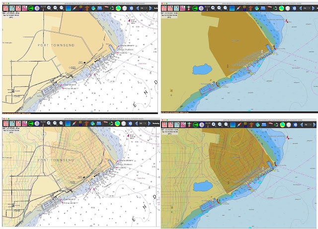
In the meantime, here is a quick look at this distinction using qtVlm simulator and live data from the Gulf Stream that I just now downloaded: GFS wind and RTOFS current.


Above is view without current and we see TW and GW are identical and both equal the wind on the grib, read from the cursor position in the status bar.

Recall that after clicking to see the image you can right click again, open in new tab and then zoom in for more detail.

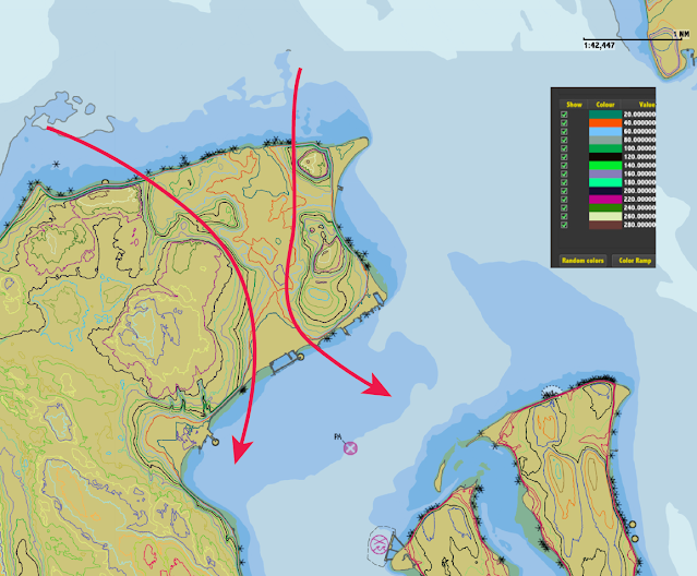
Below we add the Gulf Stream and this boat is sitting in about 3 kts at the moment.


Now we see that only the GW agrees with the grib winds and the wind directions differ by 4º and the wind speeds differ by 3 kts.  So the effect is clear, but the real value comes in analyzing the trends, which can tell us much, even if the actual values do not differ too much, but this will take me a bit longer to put together.

Another thought to address is the uncertainty in the forecasts is something like ±2 kts on the wind speed and ±10º or maybe a bit less on the direction. These uncertainties are about the level of differences in the two wind definitions in some cases—but that fact should not distract us when it comes to an effort to do the best we can in the analysis. One definition of the wind is right for this comparison and the other is not, and even though the forecasts have a notable uncertainty, that does not mean they will be wrong by that much. In short, it is not productive to ignore this distinction in wind definitions because the uncertainties in the forecast data and our own measurements might be comparable. By ignoring the distinction we increase our measurement uncertainty in a way that could be avoided.
__________

Here is an earlier article that includes the formulas we use to compute the winds, plus much discussion of the concepts in the comments.  True Wind From Apparent Wind — Revisited.


Tuesday, December 14, 2021

Adding Elevation Contours to ENC in qtVlm

One of the things we miss the most in using ENC is the essential absence of terrain info, especially elevation contours, buildings, and streets we can see from the water. There are occasional spot elevations on ENC, and even more rarely a cliff, but not much more.... and I should add here that some nations do a better job on the land than we do.  But it is generally not as good as we are used to with paper charts, and the sad part is, it could indeed be very much better—I am optimistic that the new NOAA Custom Charts (NCC) will make up for this, eventually.

A hint in that direction is the qtVlm function that lets us overlay shape files on the charts we are looking at, be they ENC or RNC.  

For an enhanced view, right click, open in new tab, then zoom in.

The top row is standard RNC left and ENC right of a chart section. Below I have overlaid streets and elevation contours....but without any enhancement. The contours are every 20 ft, which we can easily change to every 40 ft, etc; we can change the line thickness and the color bar to improve the picture. Likewise the streets are not optimized at all. This is just a quick view, but we can, as shown in the video link below, put the cursor on any contour to read its value, or on a street to read its name. You have to zoom in to see it, but we can easily identify the famous Water Street along the water in Port Townsend. 

My main goal here is to show how to get this contour data; once that is done, loading it into qtVlm is quick and easy. The process is not hard once you know the sequence. We are going for elevation contours over US lands.

How to get elevation contours

Step 1.  Go to https://apps.nationalmap.gov/downloader/

Step 2. Pan and zoom the map to the area you care about (it has a fast, positive response)

Step 3. On the top right, choose map indices = 7.5 minute, and it will draw in the areas we can select this way.  (There are ways to get larger sections at a time, up to 1ºx1º but those contour files will be 200-300MB, which are too big to load at one time. They load, but slows the program down and we never need this all at once. ) 

Step 4. Scroll the left side menu to the bottom section and check:  "Topo map data and topo style sheets."

Step 5. Check 7.5’ x 7.5’  and check Shapefile.

Step 6. At the top left Set Area of interest = Mat Extent/Geometry, then click Extent, then on the map draw a rectangle inside of what you want. Don't encompass it, but rather just have the border inside of the ones you want. (The choice will be 1, 2 or 4 or  more tiles, but we do not need to download all we select. You can also "clear Geometry and start again.)


Step 7. Back to the top left then choose Search products, and you will get a list of all the files you can download. The link is on the bottom.  Note that each tile has a name.


Step 8. You will get a file such as: VECTOR_Nordland_WA_7_5_Min_Shape.zip.  When you unzip that you get a folder called Shape that contains 180 files. We need then to pull out just the ones called Elev_Contour


Step 9. Copy these into a new folder named, say, Nordland_contours.  You can then load these into qtVlm using menu View/Shapefiles and SHOM/Open a shapefile   (SHOM is the French Hydrographic Office). In this process you direct the program to the main SHP file, but the program also needs others in this set.  You can then add multiple such files, keeping the data sets in separate folders on your computer.


Here is a quick look at elevation contours over Port Townsend area—not optimized in display, with just random colors used. But we see already something we could not see on the RNC or the ENC, namely there is a pronounced channel on the peninsula that is only 20 to 40 ft high bordered by 160 to 200 ft high hills.  This can funnel in winds creating notable wind lines at the boundaries shown here that are indeed known to local racers, which our lead weather instructor Dave Wilkinson can vouch for. He knows these waters well. Elevation contours and spot elevations on nautical charts are referenced to mean sea level, unlike the heights of lights and bridge clearances which are relative to MHW.

The video below illustrates the procedures above plus then loading them into qtVlm.


Downloading the files and loading into qtVlm (8:03)


Monday, December 13, 2021

NOAA Chart Catalogs—A Thing of the Past...Not Really

We have always praised the value of having a paper chart catalog on board as the best way to know what charts are available and a way to index what you have on board. Just annotate the catalog with a highlight marker around the charts you have.  This proved very valuable when doing a lot of sailing over several charts, or any longer voyage.

Originally, folded paper chart catalogs were delivered in great bundles to all chart dealers, who in turn handed them out to mariners who ask for them. Then as cutbacks started, this was discontinued, to be replaced by PDF versions that could be downloaded and printed or not. These could be annotated in the digital form as needed. The transition to PDF happened quite a few years ago.

But just recently, we noted that the PDFs were gone, as were previous links and web pages devoted to them.  So this is a deeper level of cutback—foretelling inevitable cuts related to paper charts, all of which are destined to be gone by end of 2024. These catalogs were all about paper charts, or the raster echarts (RNC) copied from them. Those catalogs told us nothing about the vector charts (ENC) we will all be using in a year or so. Several paper charts have already been removed... and indeed minor details are no longer being updated on the paper charts, but only in the ENC.

But we still have a couple years of sailing on paper charts where these catalogs remain valuable, which made me that much happier to discover a solution to this that will certainly take us right up to their last day on earth. The solution comes from the Coast Pilots, which we can download in full as PDFs.

Despite cutbacks in some areas, the Coast Pilots are flourishing and becoming even more important resources to all mariners, not just ship captains.  They include, for example, a complete set of the Navigation Rules, and much local knowledge on wind and current. Because some states have two Coast Pilots covering their waters, we made a Custom Interactive Index to the Coast Pilots that resolves that issue, which is not clear online.

The Coast Pilots also include all we need to create a dedicated Paper-Chart Catalog. At the end is a link to download the one we made to replace the now defunct original Pacific Coast Chart Catalog. The cover looks like this:


Each Coast Pilot has an index page showing the coverage of each chapter.


Then each of these chapters has, somewhere included, a page that shows all charts in that region. The Chapter 8 example is shown below.

Once you have these pages extracted from the Coast Pilot for each chapter, you can compile those to make the Chart Catalog.  The Pacific Coast is just 10 pages.  Then you can highlight these to mark the charts you have on board.  There are tools on line for extracting PDF pages, or just use screen caps and then print them.

This is what a page might look like once you have highlighted the charts you have on board.

Here is the Chart Catalog made as outlined above.


Once we are switched to all ENC and the new NOAA Custom Charts (NCC), which will be our paper chart replacements, we can think on ways to index these. But they will all be custom areas,  not likely following existing paper-chart borders.

For the ENC we will eventually all be using, there will then be fully reschemed ENCs that have tidy borders, scales, contours, and logical names, so it will be easy to make graphical indexes for these—but this is more or less a non-issue, in that we would most likely have all of the charts installed at all times. Looking back at that time, these paper chart catalogs will be like the plastic trays we used to organize our music cassettes.


Sunday, December 5, 2021

WAAS and EGNOS: Satellite-Based (GPS) Augmentation Systems (SBAS)

Outdoors with a clear view of the sky, we turn on the GPS and in seconds get a fix, and only periodically do we pause to be amazed at how accurate it is. To the vast majority of users, this is black-box technology. We might know that it works on a ranging principle, effectively measuring how far we are from the known positions of several satellites, and from that it can compute a position roughly like we do with radar, measuring the distances to two or three landmarks, and then plotting the intersection of these circles of position. The GPS measures the distances by timing the signals on their path from the satellite to our receiver.

Nevertheless, this is all black box. There is no way for most of us to comprehend the timing precision required (fractions of a billionth of a second), nor even how that might be achieved. It takes three satellites to get a two-dimensional fix and four to get a three dimensional fix, which is one more than we might expect, because the extra one is needed to solve the timing problem. 

Typical GPS accuracies quoted assume you have a clear view of the sky, defined as seeing all satellites above 5º high in all directions—inside or near a structure (boat!) this is never the case. Then the nominal horizontal position accuracy is quoted at about ± 8 meters. It can in fact be a bit better than that, and it can be notably less than that in real conditions. The website gps.gov is an excellent source for all things GPS. It generally has plain language discussion of most topics, followed with links to the more mathematical and engineering matters. Mariners might also look at the GPS section of navcen.uscg.gov.  The FAA remains a primary reference.  There is also an online magazine (GPS World) devoted to latest developments, often with stories and links interesting to mariners and laymen—the latest issue has links to recent EGNOS studies.

On land, GPS accuracy is not often as good as we might get at sea with a well positioned antenna. But on land or at sea anything approaching 8 meters is remarkable, being a half a boat length or less for many mariners and indeed a boat length for thousands more.

On land it can be worse when part of sky is blocked. The proof positive way to test this is just turn your GPS on and leave it running overnight, connected to a navigation program that is plotting its track every few seconds or so. Be sure the program is set to high accuracy tracking.  In the morning you will see what the spread in values is, and indeed, whether or not the centroid of that track pattern is indeed where the unit was located.

This type of test gets you two numbers. The spread in values and the distance between the mean location and the true location. Be sure the GPS and the chart you are using are set to the same horizontal datum, such as WGS 84.  

In a sense, the point at hand in this note is that if you do this test in the US or Europe with a relatively new GPS unit positioned next to the south side of a building you will likely get notably better results than you will get with it up against the north side of that building.

We can thank the aircraft industry for that as they are the ones who motivated development of a higher accuracy GPS fix so that aircraft could use it for navigation. The altitude or elevation output of an uncorrected GPS is not good enough for aviation; much of the time it is actually terrible, relative to what we can do with a modern barometer, which most all of our cellphones include.

The improved GPS signals are called "augmented," and the system in the US is called WAAS, the Wide Area Augmentation System. In Europe it is called EGNOS, the European Geostationary Navigation Overlay Service. There are also systems in India (GAGAN), Russia (SDCM), and Japan (MSAS), but we are not looking at these for now. 

There are indeed other ways to notably improve GPS locally, typically called Differential GPS;  the USCG and others have offered such services for some years. They work essentially the same as WAAS that we describe below, but on a local basis. GPS can indeed provide centimeter level accuracy with these tools, along with other enhancements, but this is another topic, beyond conventional navigation.

Yet another category of enhanced GPS performance oriented toward aircraft is called Ground-Based Augmentation Systems (GBAS), whereas WAAS and EGNOS are known as Satellite-Based Augmentation Systems (SBAS). The graphic below shows schematically how WAAS works.


Figure 1. Schematic of the WAAS system for improved accuracy and availability.

This system uses three geostationary satellites (called the WAAS satellites) located over the Equator in the Eastern Pacific (we show just one), along with some 38 reference stations (RS) scattered across North America (only two shown above), along with three master stations MS (we show just one) and six uplink antennas for getting the data back to the WAAS satellites (we show just one).

The 32 or so GPS satellites are in medium earth orbits (MEO), about 1.5 earth diameters above the surface. They are more or less evenly scattered around that shell. The three WAAS satellites, are geostationary at 2.8 earth diameters above the surface. They do not move, remaining on the Equator at the longitudes shown in the figures below.


Surface footprints of the geostationary SBAS satellites. At the satellite locations, they would be directly overhead. At the boundaries shown they will be 5º above the horizon. These are the satellites in use as of Dec, 2021. The satellites are changed periodically, so you may see older versions online.  A satellite's PRN number (stands for pseudo random noise) such as 133 for SES-15. The NMEA satellite SBAS ID numbers are defined in NMEA sentence GBS as PRN - 87.  Thus PRN 133 goes to 133-87 = 46. This shows where the WAAS satellites can be seen, but only in the shaded areas can these be used for improved GPS accuracy, discussed later in this post. (NMEA 48 replaced NMEA 51 in May, 2022.)

The GPS fix we get without help is not as good as it could be due to small errors in the timing of the signals, precision of the satellite's ephemeris (how well we know where they are located at any second), atmospheric effects on the signal transmission, as well as the lingering problem of multipath errors when the signals reflect or diffract around objects on the way to the receiver whenever we do not have a "clear view" of the sky. All small effects, but we are considering here very precise measurements.

The system works like this: The several reference stations continually record the GPS fix they get from the satellites in view to them at the moment, which they compare to their precisely known geodetic location. The discrepancy observed is then passed on to a master station that coordinates that observation with similar ones at the same time from the other reference stations, and from this they deduce what the errors are in the signals from each of the satellites that would account for the observed discrepancy. This information is then transmitted to antennas that send the data to the WAAS satellites, which in turn sends it back down to any WAAS enabled receiver on our vessels (or smart watch!) for an improved position fix. Although it was an advertising point at one time, these days, most GPS receivers include this functionality routinely.

With WAAS in place, the nominal optimum horizontal accuracy of 8 m is reduced to about ±1 m and the vertical accuracy is reduced to about the same. On board, however, we would typically set our GPS to compute only a 2-dimensional fix, and we manually enter the elevation of our antenna. Ruling out the 3-d fix yields faster and more dependable positions.

Note too that these are capabilities of the system, viewing all the sky with presumed good geometry of the satellites. There can be times when the geometry is not as good, like doing a compass bearing fix using two landmarks that are near each other. During times when the geometry is not good,  the accuracy is not as good. This varies with time. I am not sure of the best summary, but in practice it is likely that the addition of WAAS takes a fix from a practical average of ±10 m down to ±3 m. 

In any event, being able to view a WAAS satellite not only improves the accuracy of the position by applying the corrections, it improves the number of satellites we can use, and adds integrity to the fix by monitoring the health of each satellite. It also improves the accuracy of your COG and SOG, especially at low speeds.

But for this improvement to take place, your GPS receiver has to see one of the WAAS satellites. At sea within the footprint of the satellites this is easy, but on land or on inland waters, we have to check that they are not blocked by local terrain or buildings. In short we need to know the angular elevation above the horizon of the WAAS (or EGNOS in Europe) satellites, and the direction to them (azimuth) from our specific location. 

Here is a 

LIVE INTERACTIVE WAAS SATELLITE CALCULATOR

Sat Lon is the longitude of the WAAS or EGNOS satellite, from the table above. Ship Lat and Lon is the observer's position.  Elevation is the angular height of the satellite above your horizon viewing in the true direction Azimuth. Enter the data then press Calculate.

Example: to see WAAS satellite 46 from the Pacific Northwest (47.8 N, 122.3 W) we must be able to see the sky in direction of 189 T at 35º above the horizon. That is about one third of the way up from the horizon to overhead.

You can find the elevation and bearing to any of the geostationary SBAS satellites from any location within their footprint this way,  then put this info into your logbook or memory, so you know where to look for this extra accuracy.

But keep in mind that you can see the SBAS satellites from a vastly larger area than they actually provide augmented accuracy for. Each of the systems is limited to providing accuracy data to regions that are covered by their reference stations. Outside of these areas, outlined below, you can be getting a fix from satellites that the reference stations do not see. So these services are limited to the regions shown.


The farthest north WAAS reference station in the US at Barrow, AK. I believe they all have the same design.

_________

Here is an example taken in front of our office. The GPS (Bad Elf Pro) had a good view of the sky, but not at all what is officially called  clear or full sky. 


This was a run for 3 or 4 hours. This does not show very detailed results in that it would be best to record Lat Lon every few seconds and then plot those distributions. The notable NE and SE excursions were likely just a few seconds each.  The mean location of the track seems to be roughly 5 m SW of the presumed true location, but we do not know if this OpenStreetMap is accurate. It does agree with Google Earth, but they could be from the same source. In short, it is always valid to question what we are calling the right answer. If we are using an ENC, we can look into the accuracy of the data parameter for where we are. You will find that this varies more than we might have guessed.

The more interesting observation from this has been the confirmation that only one WAAS satellite shows up at a time, even though all might be in view. In our case here, I did actually see each of them (44, 46, and 51) on different days, but always only one at a time. This seems a logical way for them to behave.

We need to look to NMEA sentence GGA to determine if the WAAS is active. Below is from a later view when it switched to 51:

$GPGGA,233533.000,4740.4708,N,12223.9031,W,2,10,0.84,46.7,M,,M,,*5B

             Time       Lat         LON    6  7    8    9  10  


6 = 2 means differential, including WAAS, or 9 meaning generically SBAS. (0 = no fix, 1 = normal GPS fix)


$GPGSA,A,3,30,13,09,14,27,04,08,07,20,05,,,1.15,0.84,0.78*00

satellites used for the fix + last 3 related to uncertainties


$GPGSV,3,1,12,07,81,021,16,30,59,286,18,09,45,155,19,08,38,091,23*73

$GPGSV,3,2,12,51,33,159,30,14,28,219,29,27,27,055,17,20,24,274,17*7A

$GPGSV,3,3,12,05,22,306,29,04,12,142,12,13,09,311,24,16,07,046,*7E

sat number, elevation, azimuth, SNR for each, 4 to a sentence.


I will return later to add more about these sentences.

_______


Reference for computing altitude and azimuth of the satellites: https://tiij.org/issues/issues/3_2/3_2e.html


Friday, December 3, 2021

Connecting GPS to a Computer

To run an electronic charting system (ECS) such as OpenCPN, qtVlm, Coastal Explorer, Expedition, Time Zero,  or any of many other fine navigation programs, in a computer requires connecting a live GPS receiver to it. Unlike tablets and phones, most computers do not include a GPS receiver, but it is easy to add one.

Note added Jan 28, 2024, about 3 yrs after this was originally published. We were surprised to learn that many of the then popular units are no long for sale. We will keep the discussions as they largely apply to replacement units, but mark the section in brackets [ ] followed by options available now.

GPS Options

There are several kinds of connections. Some years ago, the only option was via a serial port connector and this is still available, but since few computers have those connectors these days, this would be then achieved using a serial to USB converter cable. But this would likely be an old GPS if it had a serial connector on the output. These days we are more likely to have a USB connector that plugs directly into the computer, or we could use a Bluetooth connection, or a wifi connection. Or we might have a NMEA 2000 (N2K) connector, but for most computer based ECS these would need the output converted to NMEA180 and there are several N2k-USB gateways for that such as the Yacht Devices YDNU-02.

So we look here at the generic options: USB, Bluetooth (BT), and wifi. These all have options in the $100 range; there are USB GPS for about $30, and some as low as $12, and indeed there are phone apps that will transmit a wireless GPS signal to your computer for $8—or spend $40 for an app like qtVlm and you get a whole array of sensor data (position, time, heading, heel, and barometer) from phone to computer by wifi, as well as a top of the line mobile nav app.

Here are examples we know about and have tested, but there are certainly very many other options. We do not have any commercial interest in any of these products. We have pictures of these shown below.

[ •  Inexpensive USB GPS: Globalsat BU-353S4 about $30. This is probably as inexpensive as they get. Has about a 6 ft cable, and you just plug it in (and follow set up notes below). Might need a USB cable extension. They are inexpensive. These units must see as much of the horizon as possible... but can look through a glass portlight (industrial velcro!). ] See replacements such as


These are both very low cost and plenty adequate for training and backup.

[ •  Low cost Bluetooth GPS: Globalsat BT-821C We have had several of these over the years and old ones still work, but not clear if still available. Was about $50. Again, velcro to a portlight, or at home set it on a window sill.  ] A good BT GPS is always a great tool to have in your nav kit. I do not find any low cost versions, but there are still a couple good higher end units listed below.

When pulling out the old units, remember GPS technology has changed; newer units will get a fix faster, and with fewer satellites, and potentially more accurate results.  My guess is anything older than about 10 years would likely show notably less than optimum performance.

[ •  High-end Bluetooth GPS with data logger and app: Bad Elf Pro about $200. You can also just turn it on periodically without any BT or other connections to record and save nav data. Very good BT behavior and includes a basic mobile app as a back up.  Great battery life. Going sailing with friends, turn it on and tie it somewhere in view of the sky, then you can take it home and export your track as a GPX file.  This will also of course serve as a live BT GPS signal for your ECS navigation. ]. This excellent Bad Elf unit is discontinued, with only expensive units from the company that we do not need. There are though still a couple very good BT units at or near $100.

Dual Electronics We have one and they work great. Also serves as external GPS for iOS devices

Garmin GLO 2.  Have not used one, guaranteed to be excellent.

 •  Antenna mount N2k GPS with built in heading sensor: Lowrance Point-1. About $270. This is an excellent unit for a vessel. We have had one for a couple years now, super fast connections.  It connects to a N2k backbone that includes the USB gateway that links it to the computer. 

There are several related units at West Marine. Many made to connect to AIS or radio, so we need to add connector adapters.

Garmin GA38 Just $78. Includes a long cable, but with BNC (coax) connectors at each end, so you will need to go from BNC to USB to get into the computer. 

 • Handheld dedicated GPS unit: It may take some research, but some of these can be wired to your computer to use as a primary source of GPS.  We have many of these dating way back, but the example we use here is our Garmin GPSMAP 78s. This is an old one, it was one of three used by team MAD Dog when they set the record for the R2AK in 2016—we had the pleasure of working with them in preparation for the race. Connecting these hand held GPSs to the computer can take some research. It is usually not covered in the manuals. We explain below how to do it with this one.


•  An iOS App that broadcasts GPS signals to your computer from your phone is GPS2IP. There is a well documented free version for testing (4 minutes at a time), and then $8 for full version with no time limits. It is best to test the free app to be sure all works as you expect, before the purchase. Our experience is it works great.  The app can be set up to transmit other phone sensor data, but at present it is position and heading. These connect via a wifi link, either TCP, UDP, or Socket, as explained in detail at their website, which also includes step by step instructions for actually connecting to most of the popular navigation programs. The app will transmit in the background, but running the GPS and broadcasting data are a heavy battery draw, so the unit must be either plugged in or not far from it.

•  The mobile version of qtVlm both iOS and Android will also broadcast the GPS signals to your computers via wifi. It has a demo version, but for this function we need the paid version, which is $40. The app will also transmit your barometer, heading, and heel, all obtainable from sensors in the phones. It will also run and transmit this data in the background, but as noted above, this is a heavy battery draw, so the unit has to be plugged to power.  But with this, you have a full navigation system in the phone, plus a backup way to send signals to your computer. A BT or USB device is likely best choice for regular usage.

Wired GPS connections

The above are sample sources of GPS and other NMEA data we can use, now we take a look at the actual connection, and for this we will use qtVlm as a typical ECS to show the process. This is essentially the same for all ECS, once you find how you access NMEA connections. In OpenCPN it is Setup/Connections; in Coastal Explorer it is Settings/Electronics; in Expedition it is System/Instruments, and so on.

Below shows the units we used for the input testing.


These are, left to right, Lowrance Point 1 antenna mount (connected by wire to the N2k backbone shown below, which in turn was connected via USB to the computer), an iPhone with qtVlm mobile app running and broadcasting GPS and other NMEA data to the computer by wifi, above it an old Globalsat bluetooth GPS, and next to it is a new Bad Elf pro Bluetooth GPS; above it is a Globalsat USB GPS; then the Garmin GPSMAP 78s, which is connected to the computer with a custom Garmin cable; below that is another iPhone, this one running the GPS2IP app broadcasting the GPS data by wifi to the computer; and on the right, an older antenna mount GPS from some 15 year ago. It still works but is slow.  The window faces due south, but there are large windows to the right of this pic providing a slice of sky view to the west and N-NW. You can click the pic, then open in new tab, and zoom for detailed view.

The N2k bus (backbone) we use for testing is shown below. 


The far left cable is the Lowrance Point 1, next to it is the YD Gateway that can be configured to output the N2k signals or convert them to NMEA 0183 which are needed for many if not most stand alone ECS. The output cable is USB. Next to that is a YD N2k barometer, followed by the 12V power connector.  We have a review article called Introduction to NMEA 2000 with a Refresher on NMEA 0183.

qtVlm connections

That is the hardware we use, now we can look at the connections. In qtVlm this is at Preferences/NMEA connections, which brings up the window below (in Windows this is Configuration/NMEA connections).


Here is the incoming setup. qtVlm can export this data to another device (Output tab), but we are not covering that here. Recommend leaving Automatically start NMEA in the Off position for training. Underway this would be turned on.

We look at the port options below. The NMEA signals will always be: 4800, No parity, 8 bits, 1 stop bit, and no control. No need to change any of these.

The Replay file is a way to view NMEA data stored in a file, which we don't cover here. (We used this function to reenact the grounding of the Ever Given in the Suez Canal.)

Edit custom serial ports is a function for Linux users. Not needed here.

Next is option to set up 3 different serial port sources (USB or BT), which we could then switch with a click. Only one at a time is used. Also not difficult to change one as needed.

If your device (i.e., tablet or phone) has an Internal GPS, this is where you turn it on. This would be for those running the mobile version of qtVlm.  Next to that is the option to Send to NMEA outputs, again not covered here—this is covered in the Wifi GPS section below.

RMB is a NMEA sentence that describes the active waypoint. This is left off. It is an option to let some external device determine what the active waypoint is. 

Display raw NMEA data  I prefer to leave on for training as it is a quick way to note we are getting signals, and it is easy to shut off.  

Record NMEA data only applies to real NMEA signals, not simulated. You can if you like record a day's sail or a race or a practice maneuver, and then replay to study it... or to gather information to improve your polar diagram.

Date and time from NMEA is useful when away from any network for an extended time. Not needed on shore with your computer connected to the internet. This automatically keeps your local computer time  up to date. Offshore, however, your computer is just another quartz watch, which will gain or lose time.

What you see when you drop down one of the serial port input options is typically a list of not just the active ports, but all the ones you have looked at recently. On a PC these will show up as a list of com ports, as shown below


For the direct USB cable plugin the process is usually just plug and play. With PC connections, the com number is typically unique to specific USB input plugs, with one, for example, called com3 and the one next to it com4, and on the other side of the laptop com5, etc. It can be valuable to use the same input for the same device to save having to reconfigure screens like the one above.  These com numbers can also change if you connect multiple devices. 

For the Bluetooth and wifi connections, there are usually a couple steps to follow in the correct order, which we come to below.

How these serial ports show up in a Mac is always a surprise. Below is what we see on an iMac after using several of the GPS sources shown above. In the Mac version of qtVlm you will see two basic forms: cu.port-name and tty.port-name. You can use either one for the input. Other Mac nav programs may only show the cu.port-name.  I think we see both in qtVlm because it offers the option to export the data as well as import it.


The green symbol on the right is a NMEA sentence filter. Most ECS have this option in some form. In this case it looks like the following, where we compare the Display raw NMEA data window, before and after applying a filter. This option is not often called for. You may have the same data from two sensors whose sentences can be identified, and this way you can shut one off.


Once the GPS, or NMEA stream more generally, is connected you can view the quality of the GPS data from the NMEA tab in the Dashboard. Start the NMEA and then press GPS status to see something like this:


I have to say "something like this..." because this is artificial in that you cannot see the two color panels at once; it is one or the other. This shows the satellites being used for the fix. The numbers are the actual satellite numbers; this is not just counting them.

Latest build of qtVlm also now predicts satellite locations for Iridium and GPS satellites and more.

The "Constellation" view is a radar presentation showing their relative locations and elevations. The circumference is the horizon, the point overhead is in the middle. The black ring is halfway up the sky. Red means the satellite has been identified and is there, but for some reason is not being used in the fix. This information is being transmitted from the GPS receiver that is doing the fixing and then telling us this satellite information in sentences GSV and GSA. The green squares are Russian GLONASS satellites (numbers 65-88). Not all receivers are configured to use these. US GPS are numbers 01-32. Augmented GPS (WAAS) are 46, 48, 44, and provide highest accuracy, but these geostationary satellites over the Equator are not easy to see on land at higher latitudes, as buildings or terrain to the south may block them out.


Video demo of connecting a wired GPS to qtVlm. (7:06)

Bluetooth GPS

Bluetooth (BT) is another popular way to connect a GPS to the computer. Once set up, it generally works as well as a wired connection, but there are two extra steps to the connection: paring the GPS device to the computer and then connecting the nav app to the serial port created by the pairing. It is important to recognize that this is two distinct steps. The Bluetooth GPS may allow for paring with multiple devices, but once paired to a computer, you can only connect one app at a time to that serial port in that computer.  Other computers on the boat could connect to the same BT GPS and use it.

The paring process will typically create two ports. In Windows they will appear as two consecutive com ports (i.e., COM6 and COM7) in a Mac they appear as cu.port-name and tty.port-name). In the PC, one of them is called "incoming" and the other is "outgoing," but this is from the perspective of the device, i.e., the GPS. So we want to use the one called "outgoing." In a PC only that one will work. You can try one and if that does not work, use the other, or you can look ahead of time, from the Windows "Bluetooth & other devices" panel, scroll down to the bottom and click "More Bluetooth options," then click COM Ports, where you learn which is the Outgoing port. It will also be the one with a name.


Bluetooth in a Mac makes a similar distinction between incoming and outgoing, more basically tied to who is asking for the data, but either one will work on a Mac, so this is not a potential stumbling block... do I hear Mac users quietly clapping in the background?


Video demo of connecting Bluetooth GPS to qtVlm(5:40)

Once the connection is made via BT the behavior in qtVlm is the same as described above with the USB. If you have both BT and USB you might use two different ports on the set up page to save setting it up again.


Wifi GPS

Finally, there is a way to get GPS into your laptop navigation system that you might not have known of, namely there are a couple phone apps (iOS and Android) that will broadcast the GPS position and time data over wifi that you can then pick up with your computer. Furthermore, since modern phones also include sensors for heel angle, barometer, and heading, you can get all of that info as well. In short, with such an app, your phone is a back up navigation system!

Below are two videos showing this connection. One using GPS2IP, which is an iOS app, and the other is using the mobile version of qtVlm, which is available in iOS or Android. GPS2IP has a free demo version you can use to see that it all works. This one lets you connect for 4 minutes. The full app is $8 and it makes a permanent connection. This app provides GPS data and heading.


Connecting an iPhone GPS to qtVlm via wifi using the GPS2IP app (2:25).

You can also do this using the qtVlm mobile app for iOS or Android as shown below.


Connecting GPS and other sensors from a smartphone to a computer (10:03). The method shown using qtVlm mobile can connect to any nav program, in Mac or PC, but the example connects it to the computer version of qtVlm.

In our online course we cover use of the internal simulator for practicing with GPS and other NMEA signals including simulated depth sounding. Later we will come back and add the use of external NMEA simulators, of which there are several.

Also to follow shortly will be an article on augmented GPS signals both in US waters using the WAAS system and in Europe using the EGNOS system. Generically these are called SBAS for Satellite Based Augmentation Systems, which are ways to get more accurate GPS data. Invented for aircraft, but marine and land navigation can often take advantage of this.

_______

For completeness, we connected the Garmin 78s using a custom cable from a much older Garmin III+ unit, shown below. It splits from the 4 pin plug to a 12V power connector and to a serial connector that we then connected to a serial to USB cable. There is also a setting in the 78s called Export NMEA. Then it all (magically) worked just fine. The newer Garmin handhelds seem to mostly not have such a wired connection option, but models such as the 276CX offer both BT and wifi links to a PC so they would serve as a backup source for the ship's electronics if needed.


If you have one of these older popular handhelds, which do in fact still work well, you can find a direct 4-pin to USB cable from third parties online, but it would be worth checking with the sellers about your application, to be sure the power and the data are wired as you need.


Friday, November 26, 2021

Sub-millibar Pressure Patterns, Part 2.

In a recent note (Atmospheric Pressure: Look Close to See its Microscopic Pulse) I presented high-resolution results of three barometer sensors in three phones here in the office using our Marine Barograph app. This app is well designed to measure and record small changes in the pressure, and indeed we saw small oscillations in the pressure that were observed on all three, presumably independent devices. 

The question was raised as to whether there could be any ambient interference with the pressure or electronic circuits inside the room that were responsible for these oscillations, so we decided to move the three phones outside and then put them into a metal box, that serves as a Faraday cage that blocks out wireless interferences. Also these were now running on batteries not connected to chargers as the first measurements were, which does indirectly link them via the ground line at least.

This new sophisticated (!) set up is shown below.


We let the units collect data for 40 min or so, and then we used the app's export .csv option on the 30-min files for each, which includes the pressure every second. These data where then imported to Excel, trimmed to be the same start and stop times, and again shifted one of them that did not have its offset turned on, as earlier.  The results are as shown below, which we annotated with the colors.


We learn a lot from this result. First, it looks like what we saw earlier measured indoors, namely about 0.1 mb oscillations at about a 70-sec period was somehow unique to being indoors and connected via the ground connection. All three showed that pattern on some level and they were more or less in sync. I believe now that this was an electronic cross talk between the green one above and the other two. That sensor circuit seems to be defective on this very low background level, and that oscillation is almost certainly artificial.

Second and foremost, however, is that within the clean environment of these new measurements, there is still a real, physical variation of the pressure on a sub-millibar level that is clearly detectable with this $15 app.  The scale of the variation shown is really small, with peaks showing up on the 0.1 mb level with periods of about 5 minutes.

It could be pulses in the actual atmospheric pressure pattern or it could be disturbances to that pattern from other sources. We see the pressure is clearly rising over this period (~0.6 mb in 26 min), and we see the rise rate increasing as well.  This is all good tactical information, totally unrelated and not dependent on any ripples in the curve. The navigator at sea would care about this early detection of a pressure rise, but does not care at all about the ripples on the curve.

On the other hand, an atmospheric scientist might care... or maybe more likely, an engineer entrepreneur might see this and wonder if that is detecting the passing of a jet plane that I cannot see or hear?  Would the military care about such a device if really works this way?  Next time you are waiting at the airport with an iPhone and this app, you can collect the data to test this WAG proposal!

We know that this app can detect wind gusts, but these are much larger spikes in the pressure on a much shorter time frame. The 5 minute period is intriguing.

In any event, it remains promising that we can purchase an app for so little that has all the functionality to be an actual scientific instrument. Crowd sourced measurements of pressure might lead to new discoveries, or at least maybe contribute to improved weather forecasting.  Mariners have no excuse at all these days to go to sea without a high precision barometer in their pocket... or as we recommend, get an old one and velcro it to the bulkhead to be aware of the shape of the pressure changes at all times.


Wednesday, November 24, 2021

Depths, Contours, Soundings, and Groundings in ENC Navigation

Electronic navigational charts (ENC) provide a vast array of safety features not available using raster navigational charts (RNC), the echart equivalents of paper charts. These notes explain how charted depth information can be used in an electronic charting system (ECS), and in particular how qtVlm is well designed to study and practice these features using its built in NMEA simulator for power or sailing vessels. It is a good representative of any high-featured ECS. We use it in our forthcoming course on electronic chart navigation.

The subject is tied to how ENC present depth contours and soundings. Indeed, the proper use of depth contours is a key to good work with ENC. To be more precise, we are not really talking about properties of the ENC themselves, but rather, what ECS such as qtVlm can do with the specified format of the ENC sounding data in compliance with recommendations of the IHO and IMO

These two organizations call for the definition and use of three specific depth contours, and all modern ECS use these conventions. The user defines in the program preferences the values to be used for each of these contours, keeping in mind that they can be changed at any time to match the location and navigational goals of the vessel, as well as the scale of charts available. The three are Shallow water contour, Safety contour, and Deep water contour.

Shallow water contour

The shallow water contour is defined as marking that depth where the vessel will certainly go aground. It would typically be the draft of the vessel, perhaps modified by the range of the local tide. The working assumption is if you cross that contour you go aground, but there are important differences between the one requested, the one displayed, and the one that triggers alarms, as discussed below.

Safety contour

This is the most important of the three. It is intended to mark the boundary of guaranteed safe water for the vessel, meaning if the vessel remains outside of the safety contour they have no worries about grounding. This contour will be highlighted on the chart with a thicker, darker contour line, and its depth value is used to identify any isolated obstruction outside of the safety contour with the prominent isolated danger symbol (magenta circle with a transparent bold X inside) if its sounding is less than the safety contour depth you requested.


The safety contour will also be marked by two different water colors on either side, which will be true regardless of whether the mariner chooses a 4-color water pattern or a 2-color water pattern. The IHO and IMO also require that the COG predictor line (or anti-grounding cone) also trigger an alarm if the predicted vessel position crosses the safety contour.

Generally the safety contour would be chosen to be the draft of the vessel plus the user's choice of a safety margin below the keel, plus a correction for negative tides in the region. Ships and other large vessels also add a correction for maximum squat they might expect.

Safety depth

The goal of most routing would be to stay outside of the safety contour, but in some cases this must be crossed, and when doing so, special caution is required. One ENC display feature that assists with this is a 4th navigator input to the navigation program called the Safety depth.  The value of the safety depth is used for one purpose only, it tells the program the color of the soundings. If a sounding is equal to or less than the Safety depth, it should be printed in black text; if the sounding is deeper than the Safety depth it is printed in a gray color. Thus when sailing inside of the safety contour it can be easier to tell the deeper parts from the shallower. The parts deeper than the safety contour have gray soundings; the parts shallower, have black soundings.

Deep water contour

This contour choice does not directly affect safe navigation and can be used as best suits the navigator. In a 4-color system it defines the outermost color boundary. We see several formulaic guides in online articles for choosing this, but they just generate a number with no specific meaning. We have suggested two practical applications, namely mark the 100-fathom contour on a coastal voyage to avoid the sometimes confused seas and currents along the edge of the continental shelf, or set it to your preferred anchoring depth to help look for anchorages ahead. Or maybe just choose the next deepest contour beyond the active safety contour to make a progressive color pattern to the water depth.

This contour is not important, other than it should be deeper than the safety contour, which in turn should be deeper than the shallow water contour. Generally the safety depth would be equal to the safety contour value or between that and the shallow water go-aground contour.

Setting ENC depth contours: The good, the bad, and the ugly

The good part is the contours we can choose, their clear presentation, their intentions, and their interaction with the ECS are as described above, which in principle provide valuable navigation aids. We have no such options using other chart forms.

The bad part is, selecting the contours we want to use is not as easy as we might guess. In all ECS, we are given the opportunity to type in the digital values we want for each of these contours (the requested values), but rarely will we actually get what we want drawn out on the chart (the displayed values). The problem is the only contours that can be displayed are ones that are already coded into the specific ENC we are using—and the only contours on the ENC are those that are on the RNC (paper chart) it was based upon. Thus if we want and ask for a safety contour of 20 ft on a US chart, we won't get it, because no US chart has such a contour on it.  

When this happens, ECS are instructed (by IHO S-52) to find the next deepest contour included in the chart at hand, and display that one. Requesting a 20-ft safety contour, will likely lead to a 30-ft safety contour, or on some US ENC there is also a 24-ft contour (more rarely) and it would take that one. Table 1 shows the contours available on ENC.


It is beneficial to know the gist of this table, determined largely by fathom charts, but even knowing the possible contours is not the end of the story. First, not all US charts have all these contours. You might have two charts next to each other with different contours. Samples (not next to each other) are shown below using a nice display feature of qtVlm that tells us all the contours in a specific chart in view, with the active safety contour underlined.


Beyond knowing what the options are, which is easily solved with this display, there is still a nuance in asking for it that can be traced to NOAA's policy of truncating the metric conversion of depths when creating the ENC based on the existing paper chart. The details are given in our book Introduction to Electronic Chart Navigation

In short, if you want a specific US contour and you have the ECS display set to feet, you must ask for something a foot or so lower than you want. If you ask, for example, for 18 ft, it will miss that one completely because it is in there as 17.7 ft. Ask for 16 to be sure to get 18, and so on.

Knowing how this works, one safe method is to look at the contours on the chart in use (viewed as feet  or meters) and cursor pick the contour you want as a safety contour to read its value, which in this case might well be reported back as 18 ft (or 5.4 m), but then ask for 16 ft, then look at the chart to confirm that the one you want is now bold with different colors on either side. Set to meters display, asking for 5.4 m will likely get you the one you want.

This extra concern called for in contour selection will all go away in a couple years, depending on where you are sailing. NOAA has an ongoing program of Rescheming all ENC and one of the many benefits of that program are new and consistent metric contours, as shown below.  Some areas are already completed, but others are a couple years out, as shown below.


The same considerations on setting the Safety contour digitally also applies to the Shallow Water (go aground) contour and the Deep Water (use as you please) contours.


An example of entering requested contours and seeing the consequences. Notice that soundings equal to or deeper than the Safety depth are in gray; others in black.


Subtleties in the use of the Safety Contour

The IHO and IMO require that ship navigation with ENC must offer the user the option to set alerts and alarms that will go off when the vessel approaches or crosses the safety contour. Most ECS that have this capability have also adopted this as an optional set up for the mariner. Thus they can turn on a COG predictor or anti-grounding cone and it will change color or set off some other visual or audio alert when it crosses the safety contour. You can choose to look ahead for any time interval, minutes or hours. It will also trigger when crossing any isolated danger (rock, wreck, or obstruction) outside of the safety contour whose sounding is less than the depth of the safety contour, or if no sounding is given.

This is a fine concept, but referring back to the notion of a sometimes bad aspect of the use of a safety contour, consider the case when there is not a contour in the chart that is close to what you want, and the next one deeper is quite a bit deeper than you want. When that happens, your otherwise useful alarm is now a nuisance. It is going off, for example, when you are crossing a 60-ft contour, when you have no danger at all above 12 ft, which is what you ask for.

One solution is just give up the audio alarm feature till the chart contours are more favorable, but there are other solutions that help clarify the situation.  qtVlm, for example, has implemented the system of Default Safety Contours recommended by Professor Adam Weintrit in his book The Electronic Chart Display and Information System (ECDIS): An Operational Handbook. In that system, if you request a safety contour that is 10 m (33 ft) or less and the only available safety contour in the chart is more than 67% deeper than you requested, then that selected contour is considered a default safety contour and it is marked with a less prominent line (lighter gray) than used for a closer safety contour.  It is still clearly different from other charted contours, but also different from that of a safety contour that is closer to what you requested. If the requested safety contour is deeper than 10 m, the default contour coloring is used if it is more than 33% deeper than you requested.

This is a seamless, behind the scenes enhancement to the presentation of the safety contour that reminds users when the safety contour in effect is not close to what was requested, and yet all other interactions with it remain unchanged. This is especially valuable when there is a mismatch of contours on adjacent or overlapping charts, as shown below.


Here we see a default safety contour in lighter gray in the bottom chart compared to the traditional ENC safety contour in the top chart. In both cases, we asked for 19 ft, and the top one had a contour at 30 ft, which was close enough to what we wanted to treat it as a traditional safety contour, but when viewing the bottom chart, its closest contour was 60 ft, so it gets relegated to a default safety contour status, which stands out from the other depth contours on the chart and also from the closer traditional safety contour that was closer to what was requested.

We also see here the danger cone alerts crossing the safety contour (orange) and the effective shallow water contour (red)—see related notes below. The safety contours are the ones in effect on the active charts. The orange alerts marked with yellow asterisks (discussed below) are going off because of the mismatch in contours; the COG predictor is detecting the safety contour from the adjacent chart, which can be seen on the lower chart.

Notice that soundings equal to or deeper than the Safety depth are in gray; others in black, which is a big aid when sailing within the safety contour.

Isolated danger symbol and the safety contour

Another nuance of the official safety contour procedures relates to the display of the isolated danger symbol for rocks, wrecks, and obstructions that are always underwater and lying outside of the displayed safety contour. These object symbols will change to the isolated danger symbol (prominent pink Philipps-head) whenever their known sounding is less than the depth contour that you requested, not the one that is actually displayed. Thus there is some virtue to requesting the safety contour that you really want (even though a deeper one might get displayed) and also setting the safety depth to this same depth. That way all the soundings will be black in waters shallower than that and any underwater hazard shallower than that will be danger symbols.

The ugly bits

What I had in mind as not a very pretty part of using the safety contour is the fact just mentioned that in the present state of US ENC, meaning before the rescheming is completed, we have cases where adjacent or overlapping ENC do not have matching depth contours. The above image is a good example. Different scales do not matter, but when the inherent contours differ it means the safety contour in effect can change, depending on the chart in view. The ECS is always choosing the next deeper one from what you requested if it does not find what you want, but that answer can change as you sail from one chart to the next, or you change the zoom level to change the active chart. Although this happens on other charts as well, the example shown here is an unusual exaggeration of this issue.

This problem is mitigated quite a bit with the use of the Default Safety Contour system, which alerts us to the presence of more than one safety contour, but it can still lead to unusual danger cone displays (the two with yellow asterisks shown above), because the ECS knows all the contours present on all of the loaded charts, whether or not it shows on the chart in view. It has to know that to trigger the alerts. Indeed, a great value of the ENC is you can load the ENC, and then navigate on an RNC and the alerts and alarms computed from the ENC will still be in effect. In this case it looks like the alarms are coming from the RNC, but in fact they come from the ENC below these that you cannot see.

Thus if you see your danger cone go orange in what looks like the middle of Nowhere, you can know that you are crossing the safety contour as defined on a chart you cannot see. In short, there is no safety issue here, we are just finding one of those places where the depth contours on overlapping charts are not the same. There are not many places this can happen, and in a year or so there should be none.

Danger cone alarms are also triggered by isolated dangers shallower than the active safety contour depth, so this behavior also changes in cases like this one.

Depth simulation in qtVlm

For navigation training and practice, the NMEA simulator included in qtVlm is an invaluable aid. There are several videos on the use of this tool, but for now I want to just summarize a new feature directly related to the topic at hand. That is, it will now simulate depth readings as your vessel moves across the chart. It can do this because no matter where you are on the chart you are between two depth contours (d1 and d2), and these define an ENC object called Depth area (DEPARE), which has two attributes, d1 and d2.  qtVlm simulates what your depth sounder would read by reporting back a depth of (d1+d2)/2 at all times, and you can display this in the depth meter (sounder) found in the instruments selection.

This is clearly a rough approximation, which appears as a bar graph in the histogram, with steps occurring as you cross a contour, but nevertheless this simulation can be used as a way to study depth sounding navigation as shown below.


If you had just the depth sounder trace shown above with no GPS working, you could find your position on this chart by matching the trace to your known heading and speed. This can be practiced with the simulator.

The simulator reads the depth below the location of the GPS on your simulated vessel that you specify in the boat dimensions tab (± 10 meters). These dimensions are entered in the same way they are specified if you were broadcasting your AIS location. Likewise when we get a ship's AIS signal, this is the way we learn where its GPS is located.


This shows the set up for a real size vessel icon with the GPS assigned to the starboard quarter, marked by a small red dot. The yellow dot forward, is one third of the LOA, which marks the rotation point of the vessel when turning in the simulator. The red ring with radius 10 m is effectively the simulated depth sounder profile on the sea bed. 

Going aground in the simulator

The simulator will go aground and stop the simulation whenever you cross the effective shallow water contour.  Recall from above, that if the shallow contour you request is not there, then the next deepest will be chosen for the water color change.  Also, if the exact contour you requested is not there, the shallow alarm does not go off at that displayed shallow contour and you do not go aground at that contour, but rather at the next shallower contour. In other words, if there are 5, 10 and 15m contours, and you ask for shallow at 7, then the 10 will be displayed, but you do not go aground or get the obstruction alarm until you cross the 5. 

You can test this behavior with the Rule tool. Just turn it on and extend it over the various contours or objects to see the color changes and notices. You will go aground whenever you detect a red obstacle warning.

If there are no shallow contours where you approach land, you go aground at the green foreshore, and with no foreshore, you go aground on the tan land.  With no ENC charts loaded, you go around at the boundary of the base map. There is a setting in Preferences that affects this choice, which is best set to the ENC chart borders. 

The grounding applies not just during simulation, but it is also taken into consideration when qtVlm  computes optimum routes, power or sail. Needless to say, it will not propose a route that takes you aground!  In this regard, the details can matter. If you do not have real dimensions assigned to your boat, then the grounding occurs when the vessel's GPS location crosses the shallow water contour or coastlines as noted above, but if you assign dimensions to your boat, then it is the rectangular profile of the boat that triggers the grounding. If your boat has, say, a beam of (C+D) = 4 meters, and your GPS is on the centerline (C=D), then you could drift abeam and go aground 2 m before the GPS gets there.

When running the COG predictor or danger cone, you will get an orange warning when the predicted position (which depends on the look-ahead time you have selected) crosses the safety contour, and you will get a red warning if it crosses the shallow-water contour.  If you have the audible alarms turned on with the danger cone activated, then these warnings trigger a graphic sign alarm and a sound. 

These warnings and alarms will also get triggered by crossing any isolated danger symbol or indeed any obstruction in any location whose sounding is less than the active shallow-water contour. The danger cone is the best way to afford this safety and to practice its function. The COG predictor line alone is less likely to hit the point source of an obstruction. 

You can investigate which alarms go off and when using the ruler tool, because it acts like a portable COG predictor and will go orange crossing the safety contour and red crossing the shallow water contour or any obstruction shallower than the shallow water contour.  You can sweep the Ruler tool line across an obstruction to see that alert. Orange alerts are announced "danger detected"; red alerts are announced "obstacle detected." Both can be used to trigger an extra visual and audio alarm, but the latter must be turned on manually first.

You can get realistic practice on grounding with dimensions assigned to your vessel, because then you will indeed go aground when that vessel outline passes over an obstruction whose sounding is less than the active shallow water contour. However, with the danger cone activated, you should not have this happen because it will warn you. That is why we are practicing this! Turn on a notable tidal current (Grib configuration / Corrections)  to see how this works when you are not going the way you are headed. 

To have the alerts, groundings, and routing restrictions work properly in the program, we must have the coastline detection set correctly, which is done on the ENC setup page.


If this is shut off, then the coastlines are defined by the borders in the base map, which are not nearly as accurate, and we would sail over or route over other shoalings as well. Likewise, assigning these to an ENC without it being loaded has the same effect.