Is this really navigation? I would have to say no, unless we are talking about really modern times where the navigator gets more and more involved with computer programs and computer files.
We have been working on converting weather maps to echarts, which has led us to using several open source utilities. Often free programs we download online can get corrupted or polluted by accident or some malware. Or maybe we want to send someone a file of data or a gpx file of a long list of way points or a detailed GPS track, and we worry that loading or unloading of it from an echart program might change the content of the file in some way. Or maybe you just want to send a long text document to someone and be sure it has not changed when it gets there or when it goes somewhere else.
It turns out that the tech world has a solution for this, which I suspect is well known to those who know it well. It is called the MD5 sum. It is a unique number created by an encryption program that is a fingerprint of that file.
To use it, you need a program that reads the MD5 value of a file (any file: executable, image, text, etc) and then you just use that program to read the MD5 sum of that file and post it, or tell the recipient what it is. Then when they get the file, they run it through the same program to check the values. If anything at all has changed in that file, just one dot or one space, then the MD5 sum will have changed and you will know it has changed.
This test does not tell you what has changed, but I believe there are numerous programs that will also compare files to detect the change. But for images or encrypted executables, you still might not know what has changed.
This very easy to use test is just to confirm that it has not changed. That is all.
One convenient version I have found is called WinMD5.exe. An example of the use of this is in this video below confirming the authenticity of the open source graphics program called Gimp... which we are suggesting could be useful for making BSB files from images.
Our goal is to convert weather maps to echarts for use in forecast evaluation (overlaying model forecasts) and general route planning. We started with the easy ones, namely the color maps from OPC that have a nice lat-lon grid on them that lets us scale the margins of the charts. This way we can make a prescription for doing this that does not involve trimming the charts for each conversion.
Underway, however, we are most likely to have access to the black and white tif maps that we can get from saildocs in reduced file size. The problem that comes up immediately is these maps do not have a nice lat-lon grid; it is shown only every 10º with large blank margins. Thus are simple approach of making the header files by hand does not work for these maps. I have tried numerous tricks that I thought would work around this, but none succeeded. We are standing by for an easier solution if someone has it. Just post a comment.
One approach that does work is to call up two more custom programs and built the map in several steps.
Step 1. This always has to be done: download the map and convert to a png, and read the dimensions of the chart viewed upright—we typically get the maps sideways as tifs.
Step 2. Georeference the chart and define the borders using MapCal_2, and save what it calls chartcal.dir, which is a text file you can open in notepad. This step is illustrated here:
Video Note: watching carefully you will see a blunder being made on the bottom right cal point, but it got caught and corrected during a simple check at the end.... nice to have such things to see how this works! There is also an error early on calling a png file a gif file. Unfortunately, nothing to learn from that if we rule out author evaluations.
Step 3. Use the program mc2bsbh to build the header from the chartcal.dir. The extension of the header made this way is .hdr. We need to change that to .kap before using imgkap (you could also create one with the right name, but this is just as easy).
Step 4. Proceed to convert the png to a kap file with the header just created using imgkap.
In an earlier video-illustrated post we did this making the header file by hand, which worked for easy to scale charts that have a full lat-lon grid. That does not work for these BW maps with large vacant borders and few reference lines, which is why we move to this procedure.... at least till we learn a better way. On the other hand, once you have these utility programs in a folder, it is probably fastest to use this present method for all charts.
( I should mention for completeness, that if one has the high-end navigation program called Expedition, you don't need any of this. You just import the image, georeference two opposite corners with a slick, fast interface they have, and you are done, and ready to view the map as an interactive chart. It is then saved for later use or for overlaying model forecasts, etc. One minute would be a long estimate of the time it takes from beginning to end! )
In principle, there is a package of utilities called kapgen that will do all of what we describe above at once, but I have not had any luck yet with using that.
It took long enough to learn to do what we do here that I want to document this process before I forget the details; later we might return to figuring out what we are doing wrong with kapgen.
All of these methods are described in the OpenCPN manual or FAQ, or links they provide. It seems easy enough when reading about it, but there are nuances that I hope we point out here.
MapCal_2.exe comes from installing the program SeaClear. Install the program, then look in the Programs Files directory, and from their you can make a shortcut to MapCal_2.exe for your desktop or other folder you are usin for the conversions.
-----------------
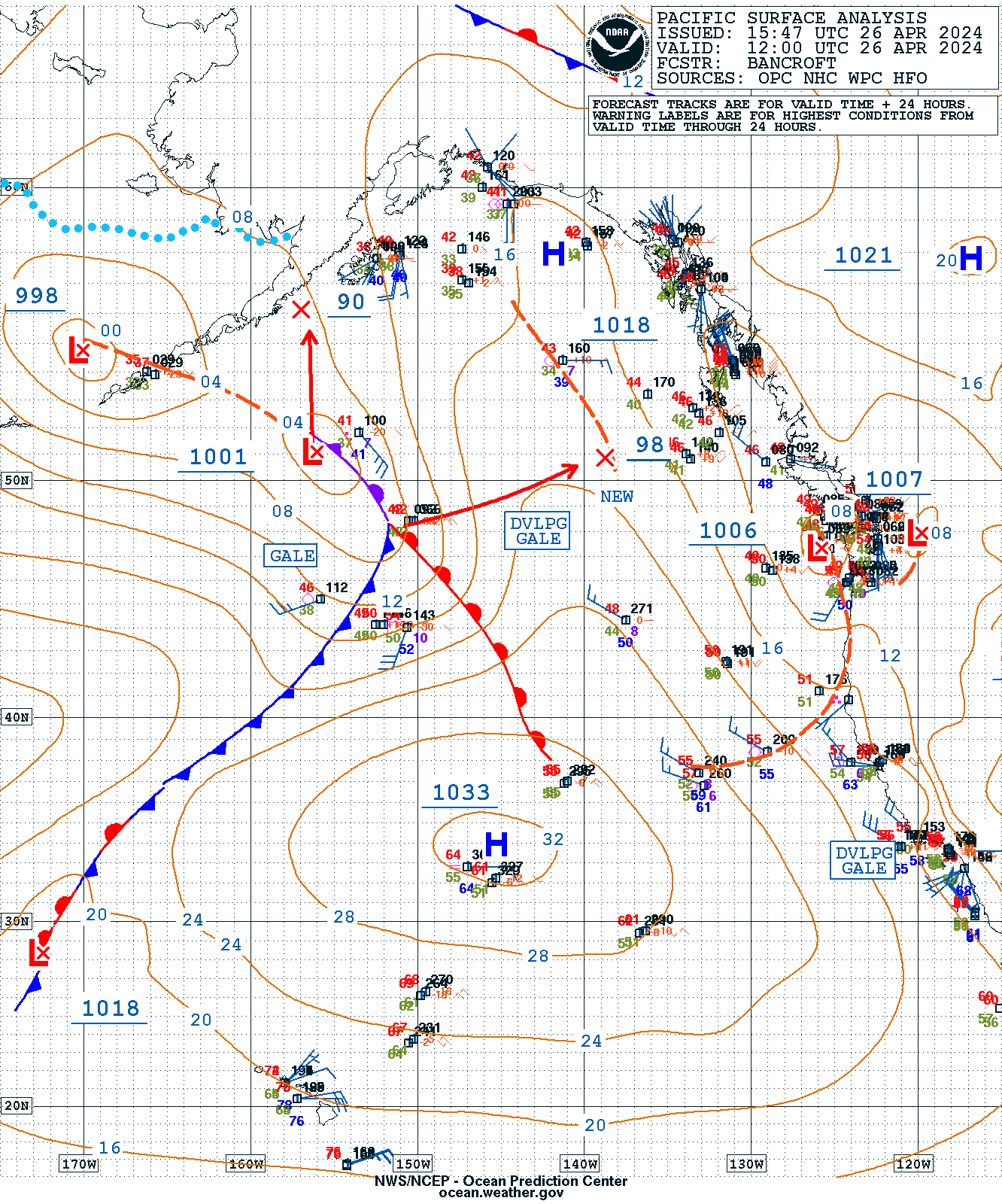
For reference, here is the header file we created for the epac surface analysis, a map that is 1446 x 1728. With this, all you need is imgkap to make a chart out of any epac surface analysis. This is for the full size maps. We need to make another one for the saildocs versions that are half this size.
! Created by mc2bsbh beta09 - Use at your own risk!
VER/2.0
BSB/NA=pyba90
NU=pyba90,RA=1446,1728,DU=628
KNP/SC=50000000,GD=WGS84,PR=MERCATOR,PP=UNKNOWN
PI=UNKNOWN,SP=UNKNOWN,SK=0.0,TA=90.0
UN=UNKNOWN,SD=none
DX=2021.6,DY=2021.6
OST/1
REF/1,126,262,60,-170
REF/2,126,1582,20,-170
REF/3,1325,262,60,-120
REF/4,1325,1582,20,-120
CPH/0.0
PLY/1,64.940016,-175.045872
PLY/2,14.3864206,-175.045872
PLY/3,14.3864206,-115.162636
PLY/4,64.940016,-115.162636
DTM/0,0
Updated May 31, to account for NOAA change in links.
When we are underway paying $1.50 per minute for satellite phone time, we clearly care if we can get the same weather map from one place that is much smaller in size than from another place, not to mention that some services might not even allow larger files to be transmitted. The latest surface analysis of the Eastern Pacific, for example, can vary from 13 to 312 kb, with multiple options in between. Again, these are the same maps.
But not only download air time matters. Storage space on our computers or tablets underway, as well as the time it takes to process the files when we look at them in different applications are also factors that make us aware of file size.
Our present project at Starpath is studying ways to get these graphic maps into an echart program (i.e. convert them to nautical charts) so we can see our precise position on the map, read precise ranges and bearings, and also to compare these professionally produced graphic products with the vectorized grib format of single numerical model predictions, such as the GFS. With the weather map made into chart we can overlay the grib forecasts right on top of the graphic forecasts.
We want to use the digital grib forecasts as much as we can because route analysis is much easier with them, We can also read digital values of wind and pressure at any point on the map—not to mention that if we are using an automated weather routing tool we must use the grib files.
But any single numerical model forecast might not be right. We need to compare them with the forecasts made by the NWS, who are looking at several models in addition to the GFS as well as other factors when making their forecasts. The pure GFS will be close to the truth much more often than far from the truth, but actual differences can be crucial in some circumstances, especially with newly developed or fast moving systems. It is simply prudent navigation to compare them on some level.
To make a chart out of a map, we first need the graphic file of the map, which leads to this topic at hand.
Our own Starpath Custom Briefings pdfs discussed below (one for the Atlantic and one for the Pacific) are very convenient ways to request any of the maps, both onland and underway, so we will look at this option after looking at the more standard sources.
We will use the 12z Eastern Pacific Surface Analysis for the example, but other products have similar results. And we list file size as downloaded—which has to be said when the options include tifs, which increase in size notably when you do anything at all to them! Some maps are presented sideways, so they have to be rotated to be read or manipulated, which if tiffs will notably increase their size, but this all takes place after they are on your computer.
Note too that capitalization of name and extension matters in the file names. NOAA now has some in color and others in black and white (BW). Below we give dimensions as w x h as viewed in normal portrait mode. Sideways means we get the map in landscape mode and have to rotate it.
Where to download the maps
The main source of weather maps is the FTP site at NOAA, all are there with a specific file name for each map along with (for some, not all) a file name that represents the latest version of that map. For example, PYBA05.tif is the 12z surface analysis of the East Pacific. It updates once a day at about 1430z to the current day’s map for 12z, but the file name remains the same. Likewise, PYBA07.tif is the map for 18z. But there is also a map called PYBA90.tif which is the latest version of this 12z analysis. It could be the 00z, 06z, 12z, or 18z map, which ever has updated the most recently. Usually we want the latest version, but there could be reasons for looking at a specific map that is outdated.
If we know the file names, we could get them directly from the FTP link. But there are several sites that index the maps so we do not need to know specific file names... but what is at the other end of these links is what we look at now. In passing, the system of keeping the same file name and updating the contents daily is a real blessing when it comes to working with these maps. Some other sources, and most European maps, have the date and time built into the file name, which really complicates any automated acquisition of them.
Starting with the neat shortcut link weather.gov/marine, which is a nice portal to all weather products, we can find the graphic map links. They link to map indexes in three different formats, but as we shall see, it is only the index layout that changes, not the maps.
Since the latest NOAA change of links, some of these notes are not valid. We need to check when we can. One path to the new map locations can be now be found from the fax schedules themselves.
So knowing the maps are the same you can choose the index presentation that best meets your needs.
These links (except for the color maps) are direct to the FTP site: http://tgftp.nws.noaa.gov/fax. The color maps seem to be a product of the Ocean Prediction Center, which I believe is where they are produced. They also provide a side link to another interactive radiofax schedule, but the maps we get there are in slightly different sizes than on the FTP site, which makes them less attractive for our purpose of making echarts out of them. Notice too that they use a different format for the file names—extensions and names all lower case.
A very convenient way to request maps on land or underway is our own Starpath Custom Briefings. These are pdf graphic indexes to each of the maps, organized by map type and forecast period, including notes on each of file size and update times. The link above explains the use of the briefings. These briefings make use of the wonderful service of saildocs.com, which reduces the file sizes by about a factor of two. This is a blessing when underway on limited bandwidth.
In the Starpath Briefings we link to the saildocs latest version of each map, which you request by email from saildocs with a single click and send. In the example we are using here, they will send back to you in return email the PYBA90.TIF that is normally 37 kb at 1446 x 1728 reduced to 18 kb at 864 x 723, also sideways. This tif format will double in size when you rotate it and save it, but it was small when you downloaded it. The reduced file size is still plenty legible, but it does not get better when the size doubles after rotating.
In a recent note I outlined how to make a BSB compatible echart from a graphic image of a weather map using a utility called imgkap. The key to that process is the header file that tells imgkap how to process the image into a .kap file that reads in an echart program.
Our goal is to provide a set of these header files covering each type of weather map so the process can be quick and painless. On the other hand, if you do want to get a little pain into the process you can see below how these header files are being made. There might even be other reasons, as something like this is required to georeference any image you might want to use for live navigation. My main goal for writing this up is to document the process if we need it later. Some of the steps took a while to figure out, and would be easy to forget.
Several details of this process discussed here are illustrated in the video below. Later we will add the most important article and video, namely what to do with these georeferenced weather maps once you have them.
We will use a Surface Analysis map for this example. Here are the steps (you might skip to the bottom for a moment to see the header file we are creating).
Step 1. Download the image. The maps we are working with now are the new (as of last 2105) color format from OPC. Some are in the png format, others are gifs. The gifs must be converted to pngs, which can be done with most graphics programs, including the stock Paint program in Windows or Preview on a Mac. Just load the gif and save or export as png.
(Later we address the black and white tiff files of the same maps. These have a few special issues to address, including rectangular pixels! )
Step 2. Read image dimensions (w x h), i.e. 1332 x 1600
In the header file, this is then RA=1332,1600
Step 3. Figure DX, DY = meters per pixel (m/px):
One approach is choose a latitude near the center of the chart, and measure the height of a rectangle some degrees on either side. For example, if 40N is in the middle, measure the pixels between 30N and 50N, i.e. 587 px. We are going to call the Lat where this is valid PP=40.
Then figure m/px from: 587px = 20º = 1200 nmi x 1852m/nmi = 2222400 m, so there are 3786.0 m/px. So DX=3786.0,DY=3786.0.
Aside: We have the option for different DX and DY values in the header. All NOAA Mercator charts have square pixels and these are the same for wx maps in png format. (Not sure yet what we will need to do here for the tifs).
Step 4. We next figure a chart scale, which is needed for the header. The concept of chart scale is transparent for RNC, which are copies of printed charts that do indeed have a scale, i.e. 1” on a 1:80,000 printed paper chart is 80,000 inches on the land. This is not so clear a concept for these weather map files that do not have a standard print size. But we do have to input a dpi for the image called DU, so once we choose that along with the DX,DY values we are committed to a scale.
The png or gif files when downloaded are likely to be at 72 dpi when downloaded on a Mac or 96 dpi when downloaded to a PC. So the 587 px we measured for 1200 nmi, would (using a Mac) correspond to 587/72 = 8.15 inches, which is = 1200 nmi x 1852m/nmi x 100cm/m x 1 inch/2.54cm = 87496063 inches, so the scale is 1: 87496063 / 8.15 = 10735713 = SC in the header.
You can do the above for whatever dpi the image comes with. It will not matter so long as we are consistent as outlined above. The dpi value is not a property of the image. It is only related to printing, which we are not doing. What we are doing is fudging a format that was intended to represent a paper chart that had known and fixed dimensions. The announcement a few years ago that NOAA was expanding all of their RNC from 250 dpi to 400 dpi was just a way to say the file dimensions (w x h) are going to be bigger.
Step 5. Now we have to figure the Lat, Lon of the corners, which involves extrapolation of the scales to project them out to the edges of the paper. (We could crop the images to the scales shown, but that would involve an extra graphics step on each conversion. Doing it this way, we have no graphics work at all once the header is in hand describing the full image.)
In this surface analysis image the Lon meridians line up nicely with the edges of the images at -175.0 to the west and -115.00 to the east. Note West Lon and South Lat are negative in this system, which is common. The top of the chart is 9 px above 65 N, and the width of 64N to 65N is 52 px, so the top edge Lat is 65 + 9/52 = 0.173, so top Lat = 65.173.
The bottom edge of the image is 37 px below Lat 16N, and the width of 16N to 17N is 23px, so the bottom of the image is at a lat of 37/23 = 1.609º below 16N, which is 14.391N.
Measuring the pixel width of the bottom margin (37 px) with the selection tool in Mac Preview (left) and Windows Paint (right). Paint does not show the bottom most line of pixels, so it adjusted up one. Step 1 in both cases is be sure the view is set to "Actual Pixels" or "Normal View." This measurement is more precise with a more sophisticated program such as Photoshop or the open source Gimp, with which you can zoom in to close view and still read the actual pixel count.
Step 6. Now we can specify both the georeference points and the chart corners, which we have simplified here by making them the same 4 points. The reference points (called REF/1, REF/2,…) can go in any order and be any number larger than 3, but the 4 corners (PLY/1, PLY/2,…) must go in order, starting at the SW corner and proceeding clockwise. (Actual NOAA RNC include a reference point for all major lights on the chart!)
Step 7. Now we can construct the header for this chart, using the standard minimum information as determined above. We will call it EPacSurfaceAnalysis. Pixel locations are referenced to the top left, with X increasing to the right and Y increasing toward the bottom.
If we name the image EPacSurfaceAnalysis.png, then we can copy this text and paste into a txt file and save it as EPacSurfaceAnalysis_header.kap, and now we are ready to make our map.
This is clearly a bit tedious, but we do not have to do this again. Once this header is made and tested we can use it as is for all East Pacific Surface Analysis maps in the future. The earlier note presented one that works with the EPac 24h surface forecast. Then getting a map into the echart program will be just download the file to the right place, run imgkap, and open the map. In fact, you can just copy and paste this text into a cmd line to get your map: imgkap EPacSurfaceAnalysis.png EPacSurfaceAnalysis_header.kap EPacSurfaceAnalysis.kap
Since posting this note (and spending much time on figuring out how to do this!) we have learned from a comment that there is indeed a very much easier way. There will shortly be here a link to a new article. The "new" method is a remarkable plugin to OpenCPN called Weatherfax, which has apparently been available for some time and I just did not know about it. It not only allows image display with convenient georeferencing, but also includes a direct link to many maps online that show up automatically georeferenced in OpenCPN.
So best bet is go the new article unless you have specific interest in the use of georeferenced images in the kap format as used with NOAA echarts.
-----------------------
With the latest surface analysis and forecast maps in an echart viewer, we can see our GPS position right on the map and plan routes across the weather patterns. It also facilitates reading wind and pressure from the map at places where none are shown. Another important application is overlaying the GFS grib forecasts on actual NWS forecasts to evaluate the GFS data—in areas where we do not have digitized NWS forecasts in the form of NDFD gribs, in which case this could be done more easily by just comparing gribs.
We discuss this in Modern Marine Weather in Section 7.2 called Georeferencing Weather Maps. In that discussion we had recommended the program Memory-Map Navigator as a way to do this as it was possible with their free, demo version. That program still has this functionality, but the demo version no longer includes this option. Other commercial products also offer this, including Ocens MetMapper, and Polar View. In principle the free program Sea Clear can do this, but I have not yet succeeded with that. All of these solutions can create a weather map echart, but they would each be unique to their own viewers. The procedure below makes a file that will open in any echart viewer.
Our electronic charting and weather training now use OpenCPN for the in class exercises, so the goal at hand was to develop a method for loading weather maps into OpenCPN. The final product should in principle open in any echart viewer. The explanation of the process is outlined below, followed by a video showing each step in action.
We will use a free utility called imgkap.exe for the PC. It is used to convert images to the .kap file format that is used in the RNC echart format, also called BSB. Once the file is made, it will open in Mac or PC versions of OpenCPN. I do not know of a Mac equivalent, but there could be something.
Below is the step by step procedure, and here is a video that shows the steps in action using a later 24h surface analysis.
Step 1. Download a copy of imgkap.exe (Windows binary, v 1.11, 3.5 MB) from dacust.com/inlandwaters/imgkap. This program is discussed at that link as well as in the OpenCPN Manual at this link opencpn.org/ocpn/imgkap.
Step 2. Make a folder on your desktop called imgkap and put imgkap.exe in it. Needless to say, you can call things what you want and store them where you want; we just need one place to put all the parts. We will need three parts: this program, the map image itself, and a header file that tells the program how to make the kap. With the nice tools made available to us, the work reduces to making the header file.... and I hope to reduce that part of the work by providing a header file for each of the standard wx maps we get from NOAA.
Step 3. Download the weather map image and save it to the imgkap folder. We use here the example of a 24h surface forecast for the Pacific, which you can get from www.opc.ncep.noaa.gov/shtml/P_24hrsfc.gif. This gif image should be 907 x 1200 pixels. The main index to all of their maps is at www.opc.ncep.noaa.gov — click the ocean tabs to get to the maps. Below is the top part of the map we are working with.
Step 4. Convert that gif to a png using a graphics program. This can be done in any version of Windows by right clicking it, choose Open With, select Paint, then after it opens Save As, choose png, save it, and close Paint. Then you will have two images in the folder a gif and an png. You no longer need the gif and could delete it.
Step 5. Now create the header file: Open Notepad and copy this text into it:
Note that the indents matter; they signify that the line above it was more than 80 characters, which is the limit. No blank lines before this text and none after it.
Then save this notepad file in the imgkap folder and name it P_24hrsfc_header.kap.
Step 6. Now we are ready to make the kap file. Now open a cmd window, ie from the Start button or equivalent type cmd and enter and the window will popup. Then type cd desktop/imgkap and enter and you should see something like this:
Then type imgkap P_24hrsfc.png P_24hrsfc_header.kap filename.kap and then enter. Filename is anything without spaces you want to name the map, ie 24h_valid_12z_jan16.kap. You can copy and paste this into the cmd window if you like with right click and paste—assuming you are using the same file names. Put another way, you can make your own generic file name convention and just use that each time as long as you have the right extensions and list them in the right order. You will get a clear error msg saying what is wrong if you make an error.
Or you can just type imgkap and enter to see the inputs and the other things you can to with this utility, ie you get a help file.
Then if you do not get error messages you will have another file in the folder called filename.kap. This is the file that will open in OpenCPN as a georeferenced wx map. Here is what you see after a successful map.
At this point, we need to just move the newly created file into a place the echart program can read it as shown in the video.
Here is what the map looks like in OpenCPN.
A final note on use of this type of home made kap file in other programs. Some echart viewers require a second descriptive file be created as well called (in analogy to above) filename.bsb. OpenCPN does not require this; it just flashes a note that there is no information on the chart. The .bsb files are relatively easy to construct from the information in the header file. I will leave that till it comes up in a specific need.
For example, one of our favorite echart programs is Coastal Explorer from Rose Point Navigation. This program does require the bsb file. These bsb files are most important for programs that are monitoring your charts to be sure they are up to date. They are also used in ECS functionality that links hotspots on the chart to announcements or corresponding Coast Pilot data and so on.
There is a note on how to make the header files here, but once you have one you can use it without knowing the details of how they are made.
Barometers and the role of barometric pressure in marine navigation have been an ongoing focus of interest at Starpath since the mid 1980s. We make books on the subject, offer extensive online training in the optimum use of barometers, and we are the North American distributors of the state of the art aneroid barometer, which is used by the National Weather Services, Navies, and individual mariners around the world.
Thus it is no surprise that we appreciate related valuable contributions to this field. One that we have known about, praised, and used for many years is the subject at hand. It came up today in class when a student was following one of our course exercises on calibrating his own barometer using online pressure resources, in particular an airport pressure reported in the form of a metar.
Essentially all airports around the world offer pressure data in this format, which is available hourly in plain language, giving sea level pressure in the form of QNH (called "altimeter" in these reports) or QFF (called "sea level pressure"). Both are pressures relative to sea level; the latter is closer to what the weather maps use, although these two pressures do not differ much unless the airport is high or the ambient temperature is extreme, or changed a lot in the past 12h. We have notes on this topic (and related one on temperature dependence of the conversions).
When we use one of these reports, or in fact any of the "official" reports, we tacitly assume the data are accurate, which is frankly—on the level we care about—not always the case. Luckily, we have a very easy way to check this, which brings us to the Gladstone Family project run by Philip Gladstone.
The Gladstone Family website is a wealth of airport weather related information, but the part we address now is his monitoring or compiling of daily accuracy records of all the pressure sensors used in the metar reports around the world. Samples below are for an airport having some troubles at the moment and one that is doing just fine.
Two reports on pressure sensor accuracy from the Gladstone Family
It is always valuable to check his report when using one of the airport stations for barometer calibration data. I wish we had such a convenient service for the buoy and lighthouse data we get from NDBC.
For completeness I should also mention our own free service for doing something similar, using all official sources, including buoys and lighthouses, as well as airport metars.
You can read about how the Gladstone Family reported accuracy is determined. As I read this, they use the same methods the NWS uses to evaluate ship and other station reports before incorporating the observations into the model forecasts.
Our free online service works differently. It is located at starpath.com/barometers. There is a detailed help file with an explanation of the process there. Briefly, we do this:
You enter the Lat-Lon of your barometer, and we find the nearest 10 stations to you that have accurate pressure online. Then you look at a plot of their location relative to you, so you can decide which 4 or 5 (or more) offer a uniform distribution of references in all directions.
At this point you could just choose the closest one and use that, but you can do very much better. Print out our form for entering pressure data for this application. Then select at least 4 of them, and go to each one and record two times and two pressures that span a time you have a pressure recorded from your own barometer. Once you have these 4 or 5 sets of data, enter them into the online version of the form and submit.
Our program will then normalize them all to a common time, and then do a least squares fit to a 3d pressure surface that spans this area, and then it drops a point at your Lat-Lon, which is equivalent to an average of all nearby sensors. This is an accurate sea level pressure value you can use for your calibration at a specific time.
But this is not yet analogous to the Gladstone Family service. So far we have only found an accurate pressure, but do not know its uncertainty. The figure below is the final output from out method, and the numbers on the right are related to this question.
The bottom line is the best estimate of your SLP at the time given. Pavg is the reported pressure at each station, normalized to the one common time. Pcomputed is the pressure we get from our computed surface at each station at this time. Delta is the difference between these two, which is a measure of how consistent that station is with its neighboring stations. If all stations agreed precisely, these deltas would all be zero.
In the example shown, we see that #1, 3, 4, and 5 are all consistent to within ± 0.5 mb, which is about all we can hope for. #2 is questionable, but OK. The one that stands out is #6, off by more than 2 mb relative to the others. When something like this is observed, we should just remove #6 from the list and do the pressure surface computation again, and generally you will see all deltas get smaller and the resulting pressure for your location will be better.... maybe not much, but better.
Thus we also have this way to check the accuracy of a pressure report, but I will be the first to agree that the neat presentation of the Gladstone Family data is extremely valuable and we are grateful for the time he has spent on developing and maintaining that fine service.
To use the Gladstone Family service, look up the 4 letter metar code for the airport in question, ie google "seatac metar" to learn it is KSEA, and then google "gladstone family ksea."


