This is a specialized technique in cel nav that is only needed when pursuing sights to their ultimate accuracy. It is on the exponential end of gaining an extra small bit of accuracy at a fairly high price in effort. On the other hand, with a systematic approach to the measurement and to the special tools required, it could be more widely used, with a corresponding rise in cel nav performance. A solar IC calculator and example are at the end here.Modern celestial navigation was well underway by the end of the 18th century. Almanacs were readily available and numerous mathematical prescriptions for doing the analysis of several sights were widely known. Newton's original invention of the sextant had pretty much replaced all earlier measuring devices, and there were several well known textbooks on navigation. A primary reference from that era was Nevil Maskelyne's Tables Requisite to be used with the Nautical Ephemeris for Finding the Latitude and Longitude at Sea. The first edition was 1766. We have at Starpath an original of the 3rd ed from 1802. That edition is also online as a PDF. It is mostly tables, but there is a short section we care about now called the "General Introduction Concerning Instruments and Observations," which is at the back of the book!
This note is essentially a reiteration of part of that Introduction on how to measure a sextant's index correction using the sun. It is no surprise that there is not much to add. Other than bringing it to light for those who have not tried it, we outline our proposed procedure and describe our work form to compile the results. This topic (and motivation for this note) came up in our online classroom discussion as we go to press with a full set of our Starpath Celestial Navigation Work Forms, which includes detailed instructions and worked examples. But this particular operation and form calls for more background than needed for the other forms, because it is the rare instance where celestial navigation can be dangerous! Our Forms booklet outlines the basics of this process, and then refers readers to this note where we fill in the background.
I will outline our procedure and show our form for this and follow up with the actual wording in the Tables Requisite to show that none of the key principles have changed. In the process we discuss the sight taking and how to build a custom sun filter for this measurement. Plus we now have a free app online that does all the arithmetic for us (linked at the end here).
First a reminder of what we are after. For the sextant to read the proper angle, the two mirrors, index and horizon, must be strictly parallel when the sextant reads 0º 0'. The sextant comes with ways to adjust both mirrors to accomplish this, but rarely, if ever, is it justified to try to get these set just right, because after each adjustment we must do multiple careful tests to confirm it, and the adjustments are interlinked. One adjustment screw moves the mirror mostly one way (think of it as a vessel motion roll), but at the same time also moves it a little bit the other way (which can be thought of as a vessel yaw); the other adjustment screw does just the opposite. In short, there is cross talk in these adjustments. The best procedure is to do the best we can to get it very close with reasonable effort, and then stop, and spend the rest of our allotted time on this to carefully measure how much it is off. Then we just correct each subsequent sextant sight for that amount. The offset is called the index error; the correction for it is called the index correction (IC). The terms are often used interchangeably, but technically they would have opposite signs... which is confusing, and we don't want confusion, so we stick with the concept of IC.
The standard way to measure the IC is to set the sextant dials to 0º 0' and then look at any distant object through the telescope. When underway, we usually look at the sea horizon, which will appear slightly split (when there is an IC needed) at the intersection of the horizon mirror (the reflected view) and horizon glass (the direct view). We then adjust the micrometer until two views of the horizon are aligned, which implies the two mirrors are now exactly parallel, and then read the dial. If we get a small reading such as 2' then this is called "On the scale," or just "2' On." In other words, this sextant read an angle when there was none, so we have to subtract that amount (the IC) from all future sights—it is like a speedometer on a car that reads 2 mph when you are parked. When moving that speedometer will read 2 mph too high.
On the other hand, if the sea horizon alignment brought the index to the other side of 0' we would read something like 58', and then we know we are 2' "Off the scale," so our instrument will read 2' too low on future sights. All celestial navigators know the jingle on how to make the correction: "If it is off, put it on; if on, take it off," because we do not want to gamble with ± signs for such an important correction. Below is a reminder of how these readings appear on the micrometer drum.

Figure 1. IC measurements. Left reads Hs = 0º 2.0', which is IC = 2.0' On. Left reads Hs = 0º 58.0', which is equivalent to Hs = – 0º 2.0' corresponding to IC = 2.0' Off. A counterclockwise (CCW) turn of the dial is in the direction of larger numbers on the micrometer, which in the telescope view brings the reflected objects down relative to directly viewed objects. We call this CCW direction "Away" as we are turning the top of the dial away from us.
The topic at hand is the reference object we use to align the mirrors. Instead of the sea horizon, it could be a star or planet, or it could be a limb of the moon. What is not often noted is that it could in many circumstances be a cloud. The alignment of any of these objects (sea horizon, star, planet, moon, or cloud, or a hilltop, a couple miles off) will indeed get us a measure of the IC, but it is not as accurate as we can do by using the sun. The sun is, frankly, the most trouble to use, but it does get the most accurate results.
"...the sun is incomparably the best object for this purpose."
—Nevil Maskelyne, 1766
Furthermore, none of these other objects gives us any direct measure of the accuracy of our IC measurement, whereas using the sun does indeed give us a check on our measurement. We can use this method to measure the sun's vertical width, which in turn we can look up in the Nautical Almanac—it varies slowly throughout the year.
The sun yields the most accurate IC, but we need very special care in the use of sextant shades or custom filters to be certain we do not get any direct look or even a glance at the sun during the process. That is the dangerous part of this technique, and probably why we do not often see this in modern textbooks or classroom courses. Even with the proper shades and filters discussed below, there can be fatigue to the eyes when applying this method, because we have to look toward the bright part of the sky frequently in order to know where to point the sextant.
Below we have a schematic presentation of the principle of what we are doing, then we look at the details of the actual measurement.

Figure 2. Schematic of a solar IC measurement. The round sun is stylized to be square so we can concentrate on the top and bottom edges. Direct view through horizon glass on the left is white; the reflected view in the horizon mirror is gray. This schematic has the suns offset horizontally, corresponding to a large side error. In practice they would be overlapped. Keeping the direct view on the left centered in the telescope, as we increase the value of Hs on the dial it brings the reflected sun down in this view relative to the direct view.
Steps 1 and 2 depict a "normal" IC measurement. With the sextant set to 0º 0', a first look shows the misalignment when an IC is needed. Bring them together turning the dial in whichever direction is needed, and then read it when aligned. The top of Step 1 would yield an IC On the scale; the bottom view would yield an IC Off the scale. Let's say our true IC is 1.6' On the scale. We might not get exactly that in Step 2, because it is not easy to judge exact overlap of two disks—keeping in mind that in the telescope view the suns are inline, not side by side as shown in Figure 2.
A better approach is the crux of this solar method. Namely we measure the vertical diameter of the reflected sun—just as we would measure the height of a star above the horizon—using first the bottom edge of the direct view sun as a horizon reference and then again using the top edge of the direct sun as the reference. This gives us two measurements of the diameter of the sun, each of which depends on the value of the IC and the sun's semidiameter (SD). With two equations and two unknowns, we can solve for both, and use the value of the SD in the Almanac as a quality check on the results.
We first use the lower limb of the direct view for a reference (Step 3), and then the upper limb (Step 4). This will give us what we call an "on scale width" and an "off scale width"—names recommended by Maskelyne in 1766. To consider actual values we would measure and record in the form, let us assume we have an IC of 1.6' On the scale and that the SD of the sun at the moment is 16.2', which is a typical value in the range of 15.7 to 16.4.
Looking at Step 3, we started 0º 0' in Step 1, we turned the dial to bigger numbers stopping at 0º 1.6' at alignment. Then we continue to bring the reflected view down by the full width of the sun (32.4'). When the top of the reflected view is aligned with the bottom of the direct view, the dial will read Hs = 34.0' (32.4 + 1.6). This reading Hs (on) = 2*SD + IC. This we call the On value of the width of the sun, which we enter in a form later.
Step 4. Now turn the dial the other direction, which moves the reflected sun up in the telescope view. This will be a rotation in the direction of smaller numbers on the dial. As we continue, we cross back over the view of Step 2 (Hs = 1.6') and then we keep rotating toward lower numbers till we are at the Step 1 view, which will be 0.0' on the dial. To align the LL we just have to rotate backward from 0.0 by an amount (32.4 - 1.6), or 30.8'. This puts us 30.8' behind 0.0', which we read on the dial as 29.2' because the dial counts backwards in the off-scale direction. In our forms, we will record the off value as 29.2 then subtract it from 60 to get Hs (off), the Off value of the width of the sun, and record it in the form. In this case, Hs (off) = 30.8' = 2*SD - IC.

Figure 2a. Dial readings for Hs On and Hs Off for the sun width measurements.
We now have two equations and two unknowns we can solve.
Hs (on): 34.0' = 2*SD + IC
Hs (off): 30.8' = 2*SD - IC
Subtract the equations to get: (34.0' - 30.8') = 2*IC, or IC = 3.2/2 = +1.6, which is on the scale. Then add the equations to get: (34.0' + 30.8') = 4*SD, or SD = 64.8/4 = 16.2'. This arithmetic is worked in the form below.
That is the principle of the measurement that leads to the design of our form for the process. The best practice, as recommended in 1766, is to do this several times and then average the results.
In our proposed method, we add one more level of organization to the measurement, which comes from our extensive work with plastic sextants. That work has shown us that the IC you measure, depends on the direction you approach the alignment from. This is a much bigger effect in plastic sextants than in a good metal sextant, but even the best metal sextant will show this effect to some degree. In plastic sextants such as the Mark 15, there is notable slack in the gears. There is much less of this in a metal sextant, but you can, for example, still often align the horizon and stop, and then make a very slight turn of the dial before you decide it is no longer as well aligned. Or align it, then see how much you can turn the dial before you note it is unaligned.
This is not just a mechanical issue, it is also related to our human interpretation of alignment. This varies between our perception of two images coming apart compared to two images coming together. Thus we recommend measuring IC in both directions. In Step 3 we rotated counterclockwise till they came apart and Step 4 we rotated clockwise until they came apart. That illustrates the principle, but not the way we recommend doing it. We want to turn the dial in the same direction for the on and off values of the alignment. In Step 3 we want to overshoot the alignment when bringing the reflected image down, and then turn the other way to align at the bottom and then top of the direct view going the same direction.
Each navigator needs to develop a way to keep track of which way they are turning the dials. What I have found useful is to think of a counterclockwise rotation to the left as "away" from me, thinking of the numbers on the top of the dial rotating away from me as I hold the sextant when reading the dials. This rotation increases the dial reading as the reflected sun moves down the view in the telescope.
With the same reasoning, I think of the other direction as "toward" me. This is in the direction of smaller numbers, with the reflected view rising in the telescope. This is clearly personalized terminology, but it helps me remember when I am turning "away," Hs is getting bigger, and the reflected sun is moving down. Others could be happier with just CW and CCW.
A first attempt at the measurement makes it very clear we have to be organized. We are turning a dial right or left, but it is backwards to us as we turn it. The motion of the sun we see is the result of a double reflection so when the numbers get bigger the moving sun is getting lower, and we are trying to keep track of its position relative to the other sun, which in principle is not moving, but the location of both of them in our view is totally controlled by very slight motions of the sextant as a whole (pitch, yaw, and roll)—not to mention that the suns are essentially the same color, and what we see at any moment would look identical to us if we did in the other direction! Pause or lose concentration for any reason, and we are lost—and must start again. Indeed, we have to know what it means to "start again." It should be no surprise that we strive to impose some order on the process.

In Figure 3 the sights start in position #1, which is what we see with the sextant set to near 0º 0' looking toward the sun (all filters in place.) We begin with Away rotations till the suns are well separated as in #4, then we start up with a toward rotation, slow and smooth till #7 and then read and record the Hs on value. Then keep going up till #9 and record the Hs off value. These are then called the "toward" values.
Next we repeat as in the bottom picture to get the "away" values, and these are recorded in the form and repeated several times as shown below.

We see from these measurements the range of variation that is observed, even in the hands of an experienced user. I must stress again that this method is not part of standard cel nav; it is a way to enhance the accuracy of sextant sights some fraction of an arc minute. I did two complete ocean passages in the 1980s by cel nav exclusively, and had never heard of this method at the time. Other factors such as good DR and logbook records are much more important for ocean navigation. On the other hand, attempts at accurate lunar distance measurements on land, should start with this method to measure the IC.
The sights are easier when the sun is lower, because we are looking more ahead than up, and the brightness diminishes with height as well, but there is a practical lower limit. An important part of this method is the check we get by measuring the SD of the sun, because we can look that up in the Nautical Almanac. If they agree we have more confidence in our data. In that comparison we make a tacit assumption that the refraction correction is the same for light coming from the top and bottom of the sun, which is perfectly valid for higher sights.
Refraction, however, changes rapidly for low sun or star heights. At Hs = 5º 0'.0 the correction is -9.9' but at Hs = 5º 32.0' (the other side of the sun) the correction is -9.1'. In other words, if we did our IC measurement with the sun 5º above the horizon, even with perfect sights we would this discrepancy of 0.8' confusing our analysis in some complex way. This discrepancy drops to 0.2' at Hs = 10º and is gone above 20º, so the practical lower limit on this method to avoid that confusion is about 20º, which is about a handwidth above the horizon.
Sextant Sun Shades and Custom Filters
...after using very many sextants of all types and price ranges, I have never seen a sextant that totally blocks out a view past the shades along one of their edges. This means that a standard sextant without a custom sun filter or eyepiece is not likely to be safe for this measurement.In some older sextants we find an eyepiece cap that is thick like a welder's glass. These are presumably intended for these solar IC sights. You cannot see anything through them but the sun, and they go on the eyepiece end of the scope so both suns get shaded this way, resulting in two suns of the same color. Sometimes a colored sextant shade can be inserted that will alter the tone or color of one of the suns, which helps when possible.
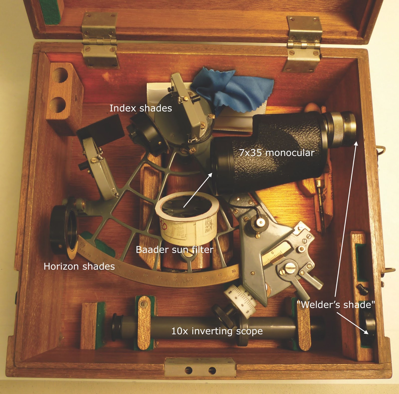
Figure 5. A Tozaki sextant with several features oriented toward the solar IC measurement. The sextant shades are crossed polarized films, which rotate for varied shading.
This sextant does include the welder's shade eyepiece that fits over the main telescope, but even with this, we need an extra screen around telescope so we cannot inadvertently glance at the sun. It is not just during the sight times we need protection; we must also lift the sextant and point to the sun, and that step also needs to be protected.
The 10 power scope is intended for IC measurements using the horizon, but this one also includes a welder's eyepiece, which must imply some optimistic thought on using it for the solar IC as well. This measurement is hard enough with a 4x40 or 7x35 scope; it takes a stronger arm and more patience than I have to succeed with the 10-power scope with its very small field of view.
The procedure for making a "Baader solar filter" for the end of the scope is given below. Figure 6 shows one way to make a simple extra screen to prevent looking around the corner of the scope into the sun as you set up the sights.

Figure 6. "It may be sometimes convenient to provide an umbrella of pasteboard, about six inches square, with a hole in the middle to receive the telescope, in order to defend the eye from the direct light of the sun, as well as from the ambient brightness of the sky, which would otherwise render this practice in many cases too painful and difficult." —Nevil Maskelyne, 1766
It could be that telescope or camera stores have ready made filters that can be used on either the eyepiece or object side of the telescope for this purpose, but we have found it easy to construct our own that custom fits the various scopes we have, which vary from 7x35 on down to a Davis 2x20. The procedure was first presented in our book How to Use Plastic Sextants: With Application to Metal Sextants and a Review of Sextant Piloting.
How to Make a Baader Sun Filter
The filter is named after the museum that originated the solar filter film we used. Alert: these films are expensive. See also links on related films as well as our earlier note on using your eclipse viewing sunshades for this—which is actually another approach, maybe even best. Make a pair of these that will stay securely in place, and do all the sights that way—short of reading the dials!
First check your sextant-telescope geometry so you know how much room you have. Generally the filter tube assembly must be made fairly thin to allow the index arm to move past it without hitting it.
Step 1. Wrap several strips of thin cardboard around the telescope, to form a small tube about 1” tall that just fits on your telescope. Glue these layers together to make the tube.

This shows the final filter, including how it started by wrapping layers around the telescope to get the right dimensions. We used our Smart Mark book marks for this, showing once again how smart they are. There is another finished filter shown in Figure 5.
Step 2. With the Baader foil between two thin cardboard or paper sheets mark the size of piece that will be needed to cover the tube and cut this out. Here we used card stock that was originally the cover of a booklet on weather.

Step 3. Make two cardboard base plate rings that have inside and outside diameters just a few mm smaller and bigger than the diameter of your tube. The film will be secured between these.


Step 4. Glue the tube to the center of one of the rings. Below we show a pocket watch being used as a weight as this glue dries. We used Gorilla glue, that dries white in 15 min or so.

Step 5. Put a trimmed layer of double-sided adhesive tape on the top of the ring. This will be used to hold the foil on the end. (We use this because we could not find any glue that would stick to the foil.)


Step 6. Carefully place this adhesive side down onto the foil to stick it to the ring, then add the second ring on top of that using the same adhesive tape to protect the edges of the foil. Small wrinkles in the foil will not matter, but you can usually do this with very few wrinkles.
Step 7. Trim the edges of the rim as much as you can, and be sure that at least one orientation of the filter will allow the index arm to pass below it. We found that the best scissors for trimming the foil, tape, or final mount are (inexpensive) cuticle scissors.

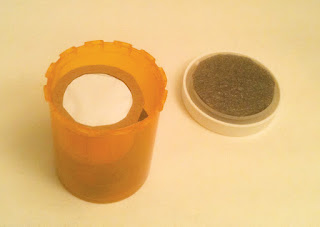
Step 8. Look for some fortuitous container that can serve for storage and protection. We found a plastic pill jar just right for this one, with a few pieces of foam inserted to hold it in place.
With one of these filters on the end of the telescope and one of the extra screens mounted around the body of the telescope you are protected during the process.


Here is a video illustration of how the suns look through a telescope with sun filter in place, along with a few other comments on the process.
The video failed to show what it looks like to rock the sextant, which is illustrated in the image below. The effect depends on the extent of side error, but we are assuming we remove side error for this measurement. Generally you can tell the vertical alignment of the suns rather easily. The main thing to catch is if they are not one on top of the other, then you need to rock (roll) the sextant to them in line.

Note that the alignment does change when they are not vertical.


With one of these filters on the end of the telescope and one of the extra screens mounted around the body of the telescope you are protected during the process.
Nevil Maskelyne's 1802 Tables Requisite original instructions for the solar method
and need for both filters.
and need for both filters.


Here is a video illustration of how the suns look through a telescope with sun filter in place, along with a few other comments on the process.
The video failed to show what it looks like to rock the sextant, which is illustrated in the image below. The effect depends on the extent of side error, but we are assuming we remove side error for this measurement. Generally you can tell the vertical alignment of the suns rather easily. The main thing to catch is if they are not one on top of the other, then you need to rock (roll) the sextant to them in line.

Note that the alignment does change when they are not vertical.
Here is a calculator for quick solutions. It is also located at starpath.com/calc.


