Battery Life of Phones Running Location Services

Phones and tablets are often valuable backup navigation systems, with many excellent navigation and weather programs available such as qtVlm and LuckGrib. It is known that location services, which we must turn on to access the internal GPS, cause an enhanced drain on the battery. Here we look into how much of a drain is this.

The topic came up again as we introduced the new low-cost miniature AIS called dAISy that will not only run in any computer-based nav program, but it will also work plugged into an Android phone or tablet running qtVlm. The battery-life question then extended to how much more of a drain will it be to run this AIS in a phone, which will be on top of the drain from the required location services.  

Below we see the battery drain with with dAISy being fully powered by an Android phone along with qtVlm.

Figure 1. A new Galaxy A03s Android phone running both qtVlm and the dAISy plugged in and monitoring AIS Traffic without external power.

This test ended as shown when we noted that the dAISy had quit working at about 5.5 hr, although qtVlm continued to function.  We suspect that the phone shut off the USB connection at some level to protect battery life — not realizing that in this case the dAISy had in fact almost negligible effect on the drain as we see below.

Note too that this direct plugin arrangement of the dAISy is just for quick observations of traffic, up to, as we know now, four or five hours.  For continuous operation, the dAISy should be connected with an OTG adapter which allows for external power application.

To see how this differs with no dAISy, we have the data below for full navigation functions running in qtVlm but no USB attachments. 

Figure 2.  A new Galaxy A03s Android phone running qtVlm with a continuous GPS fix.

We notice here that the rate of battery life drain is essentially the same as with the dAISy attached. In short, this phone running location services and a large nav app loses battery life at about 10% per hour, with or without the dAISy attached.

This is a new phone with its new battery; older phones might not be as efficient.  Also note that this Galaxy A03s is an economical choice for a backup nav system at about $88 for refurbished unit with both GPS and a barometer... plus it will run an inexpensive AIS system.

Below is the same measurement as Figure 2 using 18-month-old iPhone 11.

Figure 3.  An 18-mo-old iPhone 11 phone running qtVlm with a continuous GPS fix.

So we see a rough generality emerging, namely the battery drain from location services in action is about 10% per hour.  This will of course have to be tested to learn what other factors may influence this observation, but at least we have a starting point.

Fast Barometer Setting in US Waters

Setting a barometer to the right pressure is not the same as calibrating it, but it is the certainly the first step, and might indeed meet many practical needs. In short, we assume that if we set it to be right at one pressure, we hope it is at least nearly right at other pressures.

Also, if the barometer is in the boat, then we know it is roughly at sea level so we do not have to worry about the corrections for elevation above sea level, which is usually a dominating factor. A barometer that is 6 ft above the water is only reading 0.2 mb lower than what it would read floating on the water.

What we need is just an accurate (official) value of the sea level pressure that we can set our own barometer to read, because our own yacht's barometer is also effectively at sea level. This is not true for a ship, were the instrument could be 80 feet above the waterline.

In the past we taught that you can get accurate pressure from various National Data Buoy Center (NDBC) or lighthouse reports, or from airports (METARS). That still works, but those data takes some steps to access and on top of that they are only updated every hour.  Thus if we are to use one of them, we have to note the time and the given 3-hr pressure tendency to compute the correction to the official reading.

We now have a much faster and easier solution. I say "now," but this source has actually been available for probably over a year now, I just had not discovered it. We get the pressure data now from exactly the same place that all mariners now have to work with to get tide and current data, namely

www.tidesandcurrents.noaa.gov.

Go to that site, click the state you are in, and then on the top right, turn Legends on  if needed, and then check Barometric Pressure and signs will pop up at the places were it is known.  These data are updated every 6 minutes, which is ideal for this operation.

Then you can either set your barometer to that pressure, or maybe better still, start a note book with the time and date and the correction you observed.  As you get more of this table filled in over various pressures, then indeed you are calibrating your barometer.  If you just set it, and do not record the correction you do not learn about the pressure dependence of its errors.

Sample barometer data display at tidesandcurrents.noaa.gov when clicking FL.

In this view there is good coverage on the Gulf Coast, but not much north of there. When this happens, try clicking another state.  

Sample barometer display clicking the state of SC

When trying all near by states does not work, then you can turn to  www.starpath.com/barometers, which covers global sources of various kinds.

This could be a great resource when sailing on other vessels and you want to check its barometer. You can read read this pressure data from your phone (tidesandcurrents.nooa.gov—we should know it by heart because it is now the only official source of tide and current data)... but if you have a phone, then you are better off using our barometer app, which you could set using this method as well.

ECS Without GPS

We might assume an electronic charting system (ECS) is only useful if we have a GPS connected to it so we can track our boat across the chart. But the main components of the system are actually the echart navigation software and a set of echarts. The GPS is just a luxury. We can do a tremendous amount of sophisticated navigation, both easily and accurately, without the GPS.

In fact, the crucial part of a well-navigated voyage is done before the boat pulls away from the dock. We can do a rough layout of the route for quick time and distance estimates, and then zoom in along the route and fine tune each of the waypoints to optimize their use underway. This usually calls for choosing them such that they correlate with good visual or radar targets along the route. Then give each waypoint a name, not just a number. 

These programs also have built-in tide and current predictions, so we can estimate anticipated speeds made good (SMG) along the route, and then print out a route plan with individual route-leg courses and distances and ETAs all tabulated. This is prudent preparation, with or without GPS to track us across the chart. All US echarts are free, so now there is no reason not to have all possible charts of interest at hand for any route. See chart download options at starpath.com/getcharts.

In this note we look at a couple ways you can navigate with echarts without relying on GPS–or put another way, if you happen to lose your GPS, don’t shut off the ECS. It remains your most convenient and accurate means of chart navigation.

Also keep in mind that essentially all ECS include some form of DR mode with which you can set the boat icon at your best estimated position on the chart and then turn on DR and set the speed to match your knot meter and heading to match what you are steering. Your ECS will then plot out your DR track. Your job is to then update heading and speed as they change. 

We look here at a couple samples of navigation that might occur on the chart in Figure 1 that we must  solve using our ECS without GPS.

Figure 1. It is night, in light fog. The boat is near buoy VD and wishes to enter Baynes Channel, about 3 miles to the West. NOAA current predictions call for a current of 1.5 kts flowing toward 135T. Broadcast Notice to Mariners has just informed us that the light on buoy VK is not showing and the buoy may be off station. We have no valid GPS signals to rely on. We have a calibrated knotmeter, compass, and depth sounder. We are left to use traditional navigation to get into this channel, taking care not to get set down onto the rocks that buoy VK was supposed to mark. We are under power at 6 kts. The magenta shade on the chart means that area is in a separation zone between two vessel traffic lanes. 

First we look at what course to steer to make good a due West track correcting for the tidal current. We know we must point into the current, but how much? We do not have the benefit of a nice COG and past track from a working GPS, so we will rely on theoretical values... and then monitor the rocks by other means. The goal is to have more than one check on our navigation at all times if possible.

Course to Steer (CTS) to Correct for Current

The solution is illustrated in Figure 2. We could do this plotting on a chart, or indeed on a blank paper using standard plotting tools, but this can be solved faster with electronic plotting tools available in any ECS. One procedure is outlined below.

Figure 2. Solution to the CTS problem, which can be worked on paper charts or on an ECS.

  

CTS Procedure

Step 1. From your DR position, draw a line in the direction you want to make good (CMG) with a length longer than the knotmeter speed (boat speed) — 270 T in this example.

Step 2. From the DR position, imagine the boat drifting with the current for 1 hour. Mark the end point of that drift on the chart — 1.5 nmi in direction 135T in this example.

Step 3. From that drift position, set your dividers to the anticipated boat speed, and swing an arc to find where your speed for one hour will put you onto your desired track. Mark that point on your desired track — radius = 6.0 nmi in this example.

Step 4. The direction of that line, drift point to intersection point, is the CTS that will maintain a CMG of 270 at a boat speed of 6 kts in a current of 1.5 kts in direction 135 — CTS = 280T in this example.

Step 5. Measure the length of the line from the DR position to the intersection point and that will be your speed made good (SMG) as you crab along the the desired track — 4.9 kts in this example.

Solving this vector triangle following these steps can be done numerous ways with an ECS, depending on plotting options offered. It could all be done with one 3-leg route. 

Starting at the DR position, use the ruler tool to find a point that is farther than your boat speed in the desired direction, and drop a mark there. Then start the route at that mark with leg 1 back to the DR position;  leg 2 from there to the drift location; and finally from there find the point on the first line that is your boat speed from the drift point; and end the route there. You know the final point has to have length equal boat speed, so just monitor that read-out as you move the cursor along the line. Then use the ruler tool or measurement tool to find the lengths and directions you need.  Here is a video example of this method.

Course to Steer by Quick ECS Solution

Danger Bearings

In the above scenario, we cannot be certain that the current predictions are correct, so we need a way to monitor our progress to be sure we stay off of Fulford Reef, whose buoy (VK) is now missing. One way is to set up a danger bearing using Cadboro Point Light, which is clearly in view, near dead ahead. 

Using an ECS, we can, in seconds, measure an accurate danger bearing to the QG (Quick flashing Green) light that will keep us off the reef, as shown in Figure 3. We see that this bearing should remain less than 254 M (we are assuming a 20º E variation). We watch it with a bearing compass as we proceed, after first checking that it is now due west (250 M) as it should be. If the bearing gets smaller we are slipping north of our track; if it gets larger we are getting pushed south. If it gets larger than 254 M, we are headed for the reef, as shown in Figure 3.

Note that this type of measurement requires a good bearing compass such as the hockey puck or equivalent.

Figure 3. Selecting a danger bearing to the QG light dead ahead at the start. The 0.5 nmi range rings mark distance from the starting point, which helps for quick DR chart plotting from log readings. Note on this older chart, there was a US buoy there with name FR for Fulford Reef, but that was later replaced by a Canadian buoy VK shown in Figure 1. The reef name is also different on newer charts.

Line of Soundings Navigation

In this hypothetical situation, the only thing we have left to use is our sounder. This is not an ideal route for depth sounding navigation, but even in this case there are still a few guidelines that can assist our navigation. The main point for now is to show how powerful the ECS is for setting up sounder navigation. To do this accurately we need tide height, which we also get from the ECS program with the click of a button.

Figure 4. Corrections to be applied to the sounder readings so they can be compared to the charted depth contours. In the following, we assume these corrections were made so we are working with corrected depths.

Figure 5. A line of soundings made from an ECS program. The data can be accumulated in an automated plot or recorded by hand.  Range rings at 0.5 nmi set on the starting point helps monitor the correlation between depth and DR position. Though not the best bottom for sounding navigation, we still have a few things to note. First the depth should drop off rapidly, then carry on slowly deepening. If it should go up at about 0.5 - 0.7 nmi off (marked red in the plot), we know we are getting pushed south. Then if we are right on track, we should see the 19-fathom bump at about 1.7 nmi off (marked green in the plot)   

 ECS Line of Soundings Procedure

Whenever the water is not too deep (meaning our sounder works—often referred to as "within soundings") and not too flat, we can usually gain useful nav info from a line of soundings. Here is a fast and accurate way to set this up using ECS.

(1) Look ahead to see if depths or contours are favorable and if so choose a couple to monitor, and make rough estimates of what you expect if you are where you think you are.

(2) Check tide height to figure net correction to sounder reading, i.e., if sounder is 2 ft below water level with 5 ft of tide, then sounder reading in feet  + 2 - 5 = charted depth expected.

(3) Note time, speed, and heading, and log preferably, and start the plot of depth vs log. The goal is to have a log reading or time for each notable sounding change.

(4) After crossing the contours of interest, figure distances between key depths or contours and use ECS plotting tools to locate most likely track around the contours, as shown in the example below. Range rings on movable marks is one way to check for closest path across the contours.

 

Example of Line of Soundings Fix using ECS

With paper charts you can draw a line on transparent paper in the right orientation, and mark off the measured depths using the same miles scale as the chart.  Then slide the transparency around till you match your measurements. Line of Soundings Fix 2, is a video example of the paper solutrion.

These are just a couple chart navigation exercises that are nicely solved by ECS without GPS. There are many. Besides the range and bearing tool for standard plotting, a versatile option that is often overlooked is the ability to set multiple range rings on any mark or waypoint, or your vessel icon. This has numerous applications, we have shown only one.

The navigation procedures described here are adapted from our textbook Inland and Coastal Navigation, 2nd Edition.

Line of Soundings Fix 2

ASCAT Data in Grib Format — Gone and Back Again

Update Apr 23, 2023: Check comments at the end. Since this article was first posted, this data has come back, and then gone, and come back again. 

ASCAT is the name of a scatterometer aboard two European satellites, Metop A and B. They provide real near live surface wind observations several times a day to mariners located in any ocean worldwide. They provide the exact data we need as sailors, as if the ocean were covered with anemometers on buoys, but more important they also provide the exact data we need to verify numerical weather models such as GFS or ECMWF. The primary US source online is NOAA's Center for Satellite Applications and Research (STAR). Which shows global wind data, updated hourly in graphic format.

The introduction of scatterometer data to marine navigators in grib format came from an exclusive experimental arrangement between the Ocean Prediction Center (OPC) and the Pacific Northwest communications company Ocens, who was the sole source for this valuable data in grib format from about 2007 to 2009. In exchange for their unique access to the data, they agreed to do the custom programming to show this complex data set. At that time, they were distributing data from a specific US satellite scatterometer program, QuikSCAT, and the Ocens program ended when the QuikSCAT program ended in 2009. 

There followed a period of time with no grib access to scatterometer data, until about 2015 when the OPC made data from the new European ASCAT program available to the public in grib format for the first time. At that time Ocens offered it again, but now there were other sources, namely LuckGrib and Expedition, who both offered data downloads and display. This did indeed take extensive special programming from both of these companies, because even in grib format this data set was not at all like showing a standard wind forecast from, say, GFS.

Then, completely unannounced, in 2018 OPC discontinued the distribution of ASCAT data in grib format. Reasons for this were not clear, but we had informed hopes that the problem would be resolved. But as time passed,  it seems with COVID limiting the workforce and likely other reasons, this simply did not happen. No more ASCAT in grib format.

The digital data were still available, but no longer in grib format. It was available in a more complex format called netCDF. Scientists have viewers that show this data, but mariners typically do not.  We posted an article and video on how to use Panoply, one of those programs, but this was not a practical solution. Thus we were again with no ASCAT data in grib format.

Then in early 2022 LuckGrib took up the challenge to convert the NetCDF to grib format so it could be displayed in the LuckGrib viewer—or once downloaded from LuckGrib it could also be viewed in Expedition. So we were back with access to ASCAT in grib format thanks to LuckGrib.

But in March of 2023, NOAA removed its traditional (OpenDAP) access to the netCDF data. They simply stopped providing this data in the same way they provide all the other weather data they distribute.  In short, anyone, including LuckGrib, who might want to offer this data to mariners is once again faced with a long, complex programming job... that would  be hard to justify, especially since over the past year, the data availability had not been as consistent as it was earlier. Sometimes the data were not updated for 3 to 5 days.

In short, we are back in a mode of no ASCAT data in grib format, and this one is likely stick for a while.

It is true that this grib data have not been used as much as it should be by the overall marine community. We cannot take blame for that. For years we have taught that this is the most valuable way to check a model forecast—we have a long chapter in Modern Marine Weather on ASCAT. But it is definitely not plug and play. It takes effort to coordinate (in both space and time) when useful data are available, especially when we want to overlay the grib versions of both model forecast and an actual ASCAT measurement.

Below is a sample of how nicely and precisely we used to be able to compare forecast and measurement using grib format.

An ASCAT pass of measured surface wind speeds on July 2, 2022, downloaded from and viewed in LuckGrib. The colors are not wind speed, but rather a time scale of relative valid times. The red sector is enlarged below.

In this image from LuckGrib, the colors represent wind speeds. These actual measured winds can be (could have been!) compared with the GFS forecasted winds.  This pass took place at 1151z on July 2, 2022.

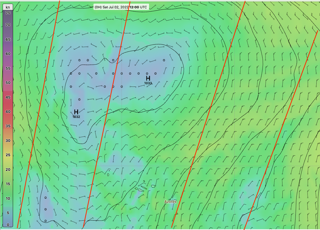
Here is the 12z GFS wind forecast for the region shown above. This comparison is within minutes, so should be good. We added the red lines so we can see where we have actual measurements.

The value of the above comparisons in grib format is we can zoom in and look at specific digital values for a precise comparison.... and indeed we see here that the GFS analysis was very good, covering a large span of wind speeds and subtle wind angle changes.  There will be times and places, where the ASCAT reveals weakness in the GFS forecasts.

So that is the type of comparison we can no longer count on.

But all is not lost... we just return to another section of Modern Marine Weather that explains how we can access the graphic presentation of the ASCAT winds with an email request at sea. Then these images can be georeferenced and displayed with the model wind forecasts overlaid on them for the same time of model evaluation. The challenges of setting up the best comparison is still the same, but these graphic ASCAT data remain available.

Programs like Expedition and qtVlm have very convenient ways to georference an image once, and then do a single button click for further updates. We have many of these georeferenced files already created, which takes that first step out of the process. 

We should also not forget  OpenCPN, which like qtVlm is free for both Mac and PC computers. It has  a very good button-click georeferencing display option in its Weather_fax plugin for the Windows version. The general grib parameter display options are not as strong as in other programs, but the key wind comparison needed for this application works well, and its image display function in the Windows version of OpenCPN is one of the best.

Below are samples of overlaying a model forecast onto ASCAT wind measurements in graphic format as a way to evaluate the model forecast. These graphic data have been dependably available for many years.

Overlaying a GFS forecast on the graphic presentation of ASCAT wind measurements using qtVlm. These are the same data shown above, but not at the same locations. The graphic files are about 37 kb so they can be requested by email. The files names and how to get them are discussed in Modern Marine Weather. We also have a video on the process.

We no longer have the digital read out of the ASCAT winds, but with little practice the color bar provided is adequate for the wind speed comparisons, where we have to accept ±2.5 kts as in agreement. Also it is important to note that the convenient grib format had a very long latency time, because it took a long time to process this data once accumulated. The graphic data, on the other hand, is updated much more quickly so we can always compare the latest forecast with an appropriate satellite pass.

Here are the various ways we can view such data in Expedition now and in the past when we had the ASCAT grib data. 

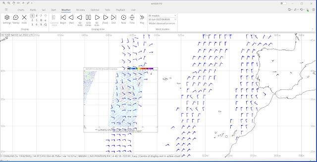
Here we see the ASCAT as grib file overlaid on one of the ASCAT graphic image files from above.

Here we zoom in to the pic above to see that the graphic data and the grib data are the same.

Here we overlay the GFS grib forecast with the grib version of the ASCAT data which was, when we had it, an effective way to check the GFS. See below

Here we zoom in to see that for the most part the model is spot on but there are regions in this complex flow of light air where they do not agree, so if we are routing across this region we can take that into account.

Finally we come to the way we will make this comparison going forward by overlaying the model wind forecast onto the graphic image of ASCAT data. Expedition has a super easy way to georeference these images since they have a prominent graticule in view.

I will try to follow through shortly and show how this can be done in the PC version of OpenCPN. 

We  have an index of ASCAT related info at starpath.com/ascat.

In the meantime, I would like to thank Craig McPheeters, author of LuckGrib, for all the fine work he put into this project over the years. It was all in the right direction.

Nick White, author of Expedition, also played a key role in this unique chapter of marine navigation history that many ocean racing sailors benefited from. Maybe one day down the line we will get this data back from the government... in some form.

The time scale is not clear, but the next generation of electronic charts called S-100 has a component for universal weather distribution called S-41X. This system and indeed all weather and environmental  data under the S-100 format will not use the grib format. They plan to use a more generalized format called HDF5. Thus if all data does indeed end up in HDF, we might get the ASCAT back in that format, which, presumably, by then we would all have nav apps that could read it.

Grib is a unique format developed by the WMO specifically to transmit weather data. But I have been assured by the WMO that they are adhering to S-100 standards when ready, and they are all HDF, not grib. I was informed that if anyone wanted grib in S-100, they can propose a change to S-100, and the next opportunity for that will be in five years. In short, they are killing their baby.

But this will be a while down the line. We might be fairly well into transmigration by then.