These are the slides with short notes and references for the video talk given at the Cruising Club of America Seminar, Feb 29, 2020. You can see these slides in the video, but they do not have the notes and live links, and are not in high res like here.

• This talk is largely highlighting topics whose details are important, which are covered in
the book.
• Link to Modern Marine Weather

• I used to say “but they are not marked good or bad," but this is no longer true as we now
have probabilistic forecasts for marine weather, as we shall see.
• We have lots of ways to check the timing of a system, mainly with pressure.
• If a forecast is in doubt then just do "half of what you want" until the next forecast in 6 hr
• We are not going to just download a GFS grib and make a decision.
2

• Both available underway by email request to Saildocs
• Learn something about the map AND something about the text
• Here we learn the speed of the high moving E
• We sail around Highs, so this is crucial info
• First 3 days of GFS is usually good, but we need routes farther, so need extended forecasts.
• Text forecasts (Storm Advisories) are especially important when dealing with tropical
storms. They are available from Saildocs.
3

• GFS overlaid onto OPC analysis viewed in Expedition compared to official Forecast
Discussion
• We want to use the digital data, so we use OPC maps to check them.
Discussion
• We want to use the digital data, so we use OPC maps to check them.
• Compare at several forecasts. ie compare 06h forecast made at 12z with the 0h
forecast made at 18z
forecast made at 18z
• Timing is everything…. GFS 0-96h is about 4h, longer forecasts add an hour
• Discussion tells which models were used and why
• Both available underway by email request to saildocs
• Auto load maps in Expedition and OpenCPN. One button click to get georeferenced maps
right on your nav screen
right on your nav screen
• Let’s look at the zoomed area
4

• Two GFS isobar parameters — needs a talk of its own!
• Viewed here in LuckGrib, which has a tutorial with references on MSLET
• Saildocs switched to MSLET as has LuckGrib. Both still call it PRMSL to minimize
confusion in display options. WRF models also use MSLET.
confusion in display options. WRF models also use MSLET.
• With MSLET we can better understand wind flow relative to isobars (gradient and
orientation)
orientation)
• Standard PRMSL is effectively an average over ~80 nmi
• Especially valuable around tropical storms… but GFS is still not dependable there.
5
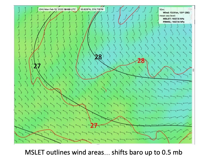
• Accounts for patches of model wind not consistent with PRMSL isobars
• Set isobar spacing to 0.25 mb and often see the trof of a front, or some indication of a trof preceding a front (squall line?)
6

the time at hand.
• This wind check process will be illustrated as we proceed
7

• Many videos and info online at modelaccuracy.com
• Calibrated instruments are crucial, as is corrections for wind heights
• Designed for analyzing Expedition log files… but could be other sources.
• N2k gateways provide ways to log wind data from any system
• Our example only with a buoy
• We added the error bars and redid the base figures
• Automated for buoys with internet connection. We have a note on how to use the buoy
function underway. Buoy reports by email.
8

• Models and forecasters do not use all ship reports. Many subtle tests applied to the reports
• Can get either map by email request. Only BW version can we get at 50% size reduction
from saildocs.
• This bottom right corner or ridge is crucial to Hawaii races, rare to have reports here
• Either one can be downloaded automatically, georeferenced in opencpn or Expedition.
• We look at the ship reports on the surface analysis for consistency.
9

• SST > 80F for hurricane.
• Stable air would make it lower; very unstable only up 10% or so, not 14 to 25.
• Curvature could raise is about 10%. But not in this case
• Ship reports can distort the isobars... ie the forecast adjusts to account for the report
• Something to think about when not in agreement.
• Cannot rely on “wind&waves” maps. Sometimes lots on barbs; more often just
those from the reports.
10

• Practice with GFS wind and pressure to see how it works out.
11

• One click download of all buoy data in Expedition... super nice feature
• Mouse over shows what you would read at NDBC
• Procedure, download the buoys then set model time to match the buoy times,
which may vary from one to the other.
• Expedition brings in latest set of buoy data but saves it when you re-load
• This will be a feature of the S-412 weather overlay to S-100 ENCs.
12

• NDBC stopped sending them to NWS. No reason given. No time for comments.
• No other NOAA source, hence moving weather data delivery to commercial third parties
• Still in FTP instructions
• We can get the data from Saildocs, one line per buoy
• Or subscribe specifying days to send, starting time UTC, and hourly interval
• Saildocs has a shortcut: send buoy51000.cur, which works for most buoys but not all.
The above link covers all sources as well as land stations such as wpow1.txt
• Saildocs has a shortcut: send buoy51000.cur, which works for most buoys but not all.
The above link covers all sources as well as land stations such as wpow1.txt
13

• Server checked on the whole minute and mail sent.
14

• Includes range and bearing to report.
• Pressure in inches but we convert to mb in the GPX file
15

• Can load the GPX reports into any nav program. This example is OpenCPN
• Need to adjust GFS model time to match each report
• We can ID ships to projects when we get later reports
• Can spot isobar shifts. Use red data to figure where that isobar should be.
• Ships with full reports likely have better data… i.e., they are more careful.
• Isobars are moving west at this time.
16

• GRIB ASCAT available from Expedition and LuckGrib.
• Timing the main issue: GRIB versions are 15+ hours old; graphic index is updated
hourly, and latest pass to show up will be ~ 2.5 hr old
• Latest useful pass could be 6 to 10 hr old.
• Generally get useful data about 3 times a day, since it does not have to be where
you are to be useful.
• Bottom right is overlay with GFS in Expedition. ASCAT red, GFS black. Shows good
agreement east and west of Cabo, but very poor to the SE.
17

• Also ASCAT B and C… A plus B makes a somewhat broader swath. Mixing data
about an hour apart.
• This is a most powerful tool, but it comes with a learning curve. See textbook.
• There is also another set of sat data from Navy WindSat, but it is not often used by NWS.
18

• This is rough sketch
• Added so you can read from the slides.
• Can plan out coverage before the race or voyage, so you know specifically when new data
will be available and you can add it to your sources timetable.
19

• Omega block can last 10 days
• If a blocking High, the map will look like this tomorrow.
• Else it will likely change
• We can get these 500 mb maps from Saildocs
20

• Main reference on role of 500 mb maps is from Joe and Lee article. Online at the Mariners
Weather Log and the book by Chen and Chesneau Heavy Weather Avoidance
• Centers of Action discussed in Modern Marine Weather

• These general rules discerned from reading a lot of forecast discussions.
• Operative rule: there is no dependable rule; just guidelines.
• BUT now we have much more to work with… as we shall see.
22

• We will follow up on this example
• Let’s see what happens at about 72 hr out along a Pacific sailing route
23

• A small variation means forecast not as sensitive to input variations and thus it is more
dependable
• Large SD means forecast is not as dependable. Small input changes lead to large forecast changes.
• Now back to last slide on 500 mb indicating maybe weak forecast about 72 hr out
24

• At 44h, 68% of all winds will be within 12 to 16 kts
• Compared to 68% within 0 and 28 kts at 90h with divergence starting about 72h
• Out 84 hours out the SD blows up. Average is about same as control, but member
runs diverge a lot, meaning forecast is fragile.
• In short, after about 80 hr the forecast is likely in question.
25

26

• NBM Oceanic covers most of the globe to 20S
• Probably best extended forecast, meaning more than 3 days or so
• Maybe best on the ocean for all times. This is not clear yet. Could be GFS is best for first 3 days.
• Now look at another example first GFS only, then the blend, then the GEFS
27

but no uncertainties.
• We do see a veer when the trof the the nW crosses at 66h
• BUT that is all we see!
• Now let's look at this same forecast with NBM
28

• Then it blows up
• Forecast is weak after this point
• Now let's compare this same forecast with GEFS (ensemble)
29

• When we see both GEFS and NBM indicate weakness or strength at about the same time
and place, we are likely safe in believing it.
• Next we look are some really new resource, just one week old
30

• Extends about 400 to 600 nmi offshore.
• We see notable light patch running NE of Guadalupe Island… but no more details.
• Could be best regional model… includes HRRR and NDFD. We need to study this one in
comparison to HRRR, which we know works well most of the time to learn more about
local forecasting. We have a note online on this topic. Use of Regional Models
31

• SD in NBM v3.2 new as of Feb 20
• The light patch has good SD
• But before and after are very uncertain ± 5 kts of wind
• Next add lower valley marker
32

33

• Here we see what likely leads to the uncertainty in the forecast
• About 1,200 ft each side of 150 to 200 ft
• Channeling is very sensitive to upstream wind direction
• In short, SD has shown us where the forecast is weak… which we do not see from
any deterministic model
34

• New resources that help us evaluate a forecast.
• Note. In this study we found forecasts that differ quite notably can still yield about the same optimum routes, with different finish times. So an eye to the polar diagrams can show how sensitive the route is to the actual wind direction. But as stressed many places, the polars have to be right, or the routing has little meaning, if not a distraction. Also we obviously do not want to take risks for small gains, even though the optimum route will do so, namely go for whatever makes it faster. Thus again the value of the statistical forecasts.
Speaker's related sites:
Frank Bohlen's articles on the Gulf Stream
Ocean Prediction Center (ocean.weather.gov, Jos Sienkiewicz, Branch Chief)
Locus Weather (Ken Mckinley's weather services)
HoneyNav.com (Stan Honey and Sally Lindsay Honey's 's articles and videos)
Seattle Forecast Office (Kirby Cook, Science and Operations Officer)
Starpath.com (David Burch HQ)
References cited in discussions:
Use of Regional Models
Inverse Barometer Effect
Free Marine Barometer app (iOS and Android)
Saildocs
Expedition
LuckGrib
qtVlm
NOMADS (NCEP source of model data)
How to Obtain Custom Grib Files
How to Combine Grib Files
No comments:
Post a Comment