Practical Use of ASCAT Winds in Weather Routing

ASCAT winds are satellite scatterometer measurements of wind speed and direction on the surface of the ocean and other large bodies of water, normalized to a 10 m height. The data resolution is 25 km, which is comparable to the resolution of typical global weather models available to the public such as GFS (27.8 km) and ECMWF (44 km). New data are available typically four times a day, from various combinations of two satellites, Metop-B and Metop-C, tracking N-NE (ascending) or S-SW (descending), bringing us data from either the port or starboard side of their split data swaths. For background in ASCAT, see www.starpath.com/ascat.  There is a video at the end here demonstrating the use of the data.

Before presenting the specifics of how to use this data, let me back up a moment and put this in perspective. Wind speed and direction are the key factors in marine navigation, in large part because the wind makes the waves, which can be a hazard to any size vessel. For sailors, it is even more primary because wind is their engine. Thus this is the most fundamental information available. It is like having the ocean covered with thousands of buoys measuring wind speed and direction.  But unlike isolated real ocean buoys who give us data every 10 min in some cases, hourly at worst, the ASCAT data covers large swaths of the ocean but only give us data 3 or 4 times a day. 

In a sense, the ASCAT data have done a major job for us even if we do not look at it, because it is a crucial input to the global weather models whose forecasts we must rely on for routing. But even though the models have assimilated the latest ASCAT data, the model forecasts are not guaranteed to be correct. It is specifically not a goal of the models to reproduce the ASCAT and buoy observations. They have a broader goal to produce the best overall forecast at many levels of the atmosphere. In short, the model forecasts may in fact not be correct in some circumstances, which is why we must compare several models to decide which is likely the best.

And indeed, circling back to check a model forecast with actual ASCAT measurements at a specific place and time we care about is one of the primary reasons for us to access the ASCAT data ourselves. If one model forecast agrees with the ASCAT measurements and another does not, it is most likely the better one to use for our routing computations

Another reason to continually monitor the ASCAT wind measurements for our intended route is the occasional observation of localized anomalous flow. We might spot a notable hole in the wind or a shear line that is not apparent in the global model forecast. In these cases, we have to realize that the ASCAT are real data. That is what the wind was doing at that time, regardless of what the model might imply or not show, and we need to route with that in mind. 

The other aspect of "perspective" is to recognize that even though these ASCAT wind measurements are indeed the most fundamental data we care about, the use of this data, which takes several easy, but non-standard procedures,  is definitely in the realm of "going the extra mile" to learn the very most we can  about the wind ahead of us. For a racing sailor, this is standard operating procedure, but when cruising it would be called on less often, unless we are negotiating a dangerous wind pattern or, more likely, some light air pattern in which we are just  looking for enough wind to get there. 

We have presented this perspective in the past, and in earlier editions of our text Modern Marine Weather, but then after outlining the basic guides to getting the data by standard procedures, we moved on. Based on discussions with practicing navigators, however, it seems that we needed a more specific procedure for accessing this crucial data, and that is what we have created.

We have semi-empirically compiled graphic indexes of the available data and pass times for the typical cruising and racing waters around North America and Europe, presented below, as well as ways to automatically access the latest available data of interest. (Note that we are not covering here the even more convenient means of obtaining this data in grib format, which can be achieved with LuckGrib or Expedition. Users of those two fine apps, might still find some benefit from the timing structure we present here.)

We assigned the names to these regions; they are not official.

Each of these named regions provide a potential of 4 data opportunities in each 24 hr period, and the only way to see which might be latest data available is to download all 4 images. The file size varies from 20 to 40 kb, depending on how much data it includes. The UTC times shown (±1 hr) tell us satellite passage times of the 4 opportunities for new data. They occur in pairs, 13 hours apart, where the two passes of each pair are about an hour apart.

For example, in Biscay, we have data passes at 10:30 and 21:30, ± 1 hr. If I go to the ASCAT web site now and look at what passes took place yesterday, I get the files shown below. 

In the top we see the two passes at 21:30 ± 1h and on the bottom the two at 10:30 ± 1hr.  These are the actual live transit times of the satellites, representing the valid times of the wind measurements. On other days, these times will be different, but remain within these windows. 

But we do not get this data instantly. It takes 2 to 3 hr to process the data, so for the Biscay region, we would only look for new data at about 00:30 and 1430. Note that this delay time or latency is about the same as it is with the model forecasts, which also take 2 to 3 hr to process for our consumption in grib format. 

To clarify the concept that there will be new data about 4 times every 24hr: consider the example of San Francisco with valid times of 0525 and 1825 UTC, ± 1 hr, noting that it takes about 2 hr to process the data.

Thus while underway or planning a route across these waters, we would go to Google Earth (or wherever we are looking at the data) at about 0725 or later UTC and download all four passes given. We do not know ahead of time which of the four will bring the new data but most likely two or them will have a swath of new data that will be valid at 0525 ± 1hr. Then again at 2025 or later we would again download all four of the passes and among those will likely be two new data swaths valid at 1825 ± 1hr.

That is in effect a cookbook approach to the data, using our indexes as guides for when to look. We will not get new data between these two periods. We then have to correlate the valid times with the model times and forecasts at hand.

There are several ways to get the data underway. You can request the images from Saildocs or you can use the custom KML files we made to use in either qtVlm or the desktop version of Google Earth, which is a free download for Mac or PC. The KLM files can also be adapted for use in OpenCPN. For the last two methods at sea, we need to link our internet connection to a satphone or Iridium Go type device.  With those procedures the links can be stored in the apps and accessed with a button click.

To request the files from Saildocs, use this request structure for Biscay (green number from our index), meaning send this text in the body to query@saildocs.com (colors added to show what changes for each file, but using this method, you just need to change the 133 for Biscay to say 86 for Bermuda.

Send https://manati.star.nesdis.noaa.gov/ascat_images/cur_25km_METB/zooms/WMBas133.png

Send https://manati.star.nesdis.noaa.gov/ascat_images/cur_25km_METB/zooms/WMBds133.png

Send https://manati.star.nesdis.noaa.gov/ascat_images/cur_25km_METC/zooms/WMBas133.png

Send https://manati.star.nesdis.noaa.gov/ascat_images/cur_25km_METC/zooms/WMBds133.png

This will get you the 4 images of the data that you can then analyze manually from the graphics alone. They have a Lat-Lon grid as shown above but will not be georeferenced into a nav program. But the  main point is you can get the data that easily and our indexes show what to ask for and when.

Our ASCAT page links to articles and demos with details, plus has a link to get all of the KML files and the graphic indexes. We will add more examples as soon as possible, and in particular the process of comparing with model forecasts.

Viewing ASCAT winds in Google Earth desktop version (using the Starpath indexes above.)

Speed and Heading — Basic, But Not Always Simple

Speed and heading are two fundamental parameters in marine navigation, but as instruments and navigation programs become more sophisticated, we can face challenges in keeping these basic parameters in order.  I do not refer to speed over ground (SOG) or course over ground (COG), these one-time elusive parameters are now the simplest to understand and to measure. They come from the GPS instrumentation; meaning their abbreviations and place in NMEA sentences are all very clear.

The challenge comes with boat speed through the water (knotmeter speed) and more often with the heading of the boat, being the angle between the centerline and either true north or magnetic north. These are sensor measurements that get transmitted to the nav program via NMEA sentences or N2k parameters. 

The issue is that these parameters can be transmitted in more than one NMEA sentence, and these days it is not uncommon to have more than one heading sensor, and if these might be from different companies they might be telling you the heading in two different sentences. At that point we need to learn if the sensor software will let us choose which sentence to use, some do, some don't, or if our navigation program lets us filter out the ones we do not want—again, some do, some don't. 

That is in large part the issue. Seems simple enough, but I know from recent experience this can eat up hours of time sorting out, so these notes are an attempt to alleviate that issue—and to document the findings we needed to resolve a related case.

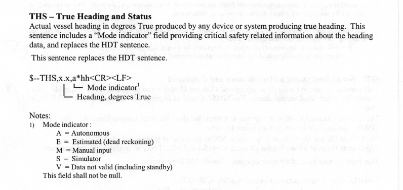
Heading is the more common issue, so we look at that first. Here are the primary NMEA sentences that involve the heading of the boat, keeping in mind that electronics can create proprietary sentences, plus some electronics still export old sentences that have been deprecated—a NMEA term meaning do not use these anymore. 

Old equipment still using HDT use it in the form: 

$--HDT,x.x,T*hh

Likewise you will also sometimes see:

$--HDM,x.x,M*hh.  Both of these are old.

When using N2k (See Introduction to NMEA 2000—with a Review of NMEA 0183) there will be a conversion between PGN parameters and NMEA sentences. The correlation is shown below as presented in an Actisense gateway manual. See a similar list at RosePoint Navigation. 

Note that the vessel heading (PGN 127250) can be exported to several NMEA sentences, which can potentially cause a conflict if other devices are also exporting the heading.  

Abbreviations in ECS

Now taking a look at how these parameters are presented in various ECS, with a note that electronic charting system (ECS) is the official name of any navigation program that is not a type-approved ECDIS. In short, any "nav program," "charting software," or console "chart plotter" interface to a GPS sensor. We cover this distinction in our text Introduction to Electronic Chart Navigation.

It is not easy to find official sources for recommended abbreviations. Bowditch, for example, 2021 edition, page 437, Glossary of Abbreviations, gives S for speed and Hdg for heading. STW and CTW are not listed. S is also used for set, south, slow, sand, and the sea-air temperature difference correction!

A more useful source is the International Electrotechnical Commission (IEC) Glossary online  where we find these definitions:

According to this important source, CTW and STW are well recognized abbreviations. Also it appears that CTW and "heading" could be used interchangeably. In principle we have a heading at the dock but not a CTW. ECS that use both (HDG and CTW), such as qtVlm and Expedition (identifies CTW as "course"), are more general.  Some consider that CTW should be HDG + leeway, but this is just the sort of thing that has to be sorted out within the ECS in use.

Looking at the speed parameter, that can be made complex as well. Generally we think of STW as the speed in the direction we are pointed, our HDG, but if we have much leeway it will reduce the proper knotmeter reading, as shown below and discussed in Leeway effect of knotmeter speed.

New age instruments

There is every reason to be sure to have a traditional paddle wheel knotmeter as well as both a magnetic compass and a magnetic heading sensor on the boat, but with those in place we can improve on both with new GPS based sensors, often called "satellite compass" or "satellite speed log" and indeed some provide both data and more.

A single GPS sensor can measure SOG and COG but it has no way to know your heading, but two GPS sensors in line with the centerline, say one at the bow and one at the stern, does know your heading, which is just the bearing from your stern location to your bow location.  Two such sensors make up a "satellite compass" that can measure your true heading at any time, in addition to COG and SOG, being how the pair is moving relative to the fixed earth. The heading can also be exported in magnetic units using the USGS software program called GeoMag. It computes accurate variation based on your Lat and Lon and the World Magnetic Model, which is updated every five years. (You can access GeoMag on your phone with the USGC app CrowdMag.)

The technology for this type of instrument is well advanced; the two GPS units do not have to be on the bow and stern, they can be just a foot or so apart in a single unit. There are several models, in the $1,000 price range.  There is a lot of math involved and they do require at least 5 satellites in view for best performance. Once the heading is known, the SOG in the direction of the COG can be projected onto the direction of the heading, called the longitudinal velocity, which is the speed you are moving in the direction you are headed, and projected onto the perpendicular direction, called the transverse velocity. The latter is the speed you are moving sideways. 

Here we see that one GPS tells COG the course over ground, and we can imagine the computation of SOG as the distance between the locations at time T1 and T2 divided by the time interval (T2-T1).  With two GPS sensors we can compute HDG and then project the SOG vector onto that heading and the transverse direction.

Note that we are not measuring leeway. The instrument does not even know we are in water. When this data gets reported to us in a NMEA sentence it would likely be VBW.

We would be getting ground speeds, not water speeds. This does not help analyze leeway but could be helpful docking and it could help us interpret current sets and our thinking on the derived parameter course made good (VMC).

Furuno has an attractive advancement of this concept in their SCX 20/21 Satellite compass. They use four GPS sensors so they get more reference lines to compute around, six in principle, two fore and aft, two abeam, and two diagonal.  This way, with still more math, they can measure and account for all vessel motions (roll, yawl, pitch) and correct for them, in addition to reporting heel angle (roll).  This allows them to get good results with fewer satellites.  It is a relatively small box, with list price of about $1,400, and taking only about 2 watt of power.  We see these on several high-tech race boats.

On the left is the SCX 21 for NMEA 0183 and the one sitting loose on the deck is the SCX 20 for N2k. This image and the one below are from a 2020  Panbo review of the instrument. The latest instrument includes 2023 improvements.

The displays from the two units above. Note that the headings differ as neither one has been carefully aligned with the center line in the demo pictured here.

I do not have direct experience with this unit, but the specs and output seem impressive:

— heading to ± 1º

— accurate, stable heading leads to clean radar trails

— very high GPS accuracy of ± 5m

— SOG to ± 0.02 kt with 5 satellites

— VBW speeds to ± 0.02 kts

— rate of turn (ROT) output for AIS broadcasts

— barometer ± 1mb with calibration offset option            

— air temp ± 2ºC 

— heel output for leeway computations and anemometer corrections

— data smoothing and offsets available on all outputs

— DR mode for lost GPS signals

_______________

I have been reminded in a comment by navigator Mark D'Arcy of the related issue that ECS often have access to multiple GPS sensors, which in turn can present similar conflicts that might lead to the vessel position jumping around a bit on the screen. Most ECS and indeed all ECDIS have a means of selecting what will be the primary source of GPS and setting this will solve that problem.

Battery Life of Phones Running Location Services

Phones and tablets are often valuable backup navigation systems, with many excellent navigation and weather programs available such as qtVlm and LuckGrib. It is known that location services, which we must turn on to access the internal GPS, cause an enhanced drain on the battery. Here we look into how much of a drain is this.

The topic came up again as we introduced the new low-cost miniature AIS called dAISy that will not only run in any computer-based nav program, but it will also work plugged into an Android phone or tablet running qtVlm. The battery-life question then extended to how much more of a drain will it be to run this AIS in a phone, which will be on top of the drain from the required location services.  

Below we see the battery drain with with dAISy being fully powered by an Android phone along with qtVlm.

Figure 1. A new Galaxy A03s Android phone running both qtVlm and the dAISy plugged in and monitoring AIS Traffic without external power.

This test ended as shown when we noted that the dAISy had quit working at about 5.5 hr, although qtVlm continued to function.  We suspect that the phone shut off the USB connection at some level to protect battery life — not realizing that in this case the dAISy had in fact almost negligible effect on the drain as we see below.

Note too that this direct plugin arrangement of the dAISy is just for quick observations of traffic, up to, as we know now, four or five hours.  For continuous operation, the dAISy should be connected with an OTG adapter which allows for external power application.

To see how this differs with no dAISy, we have the data below for full navigation functions running in qtVlm but no USB attachments. 

Figure 2.  A new Galaxy A03s Android phone running qtVlm with a continuous GPS fix.

We notice here that the rate of battery life drain is essentially the same as with the dAISy attached. In short, this phone running location services and a large nav app loses battery life at about 10% per hour, with or without the dAISy attached.

This is a new phone with its new battery; older phones might not be as efficient.  Also note that this Galaxy A03s is an economical choice for a backup nav system at about $88 for refurbished unit with both GPS and a barometer... plus it will run an inexpensive AIS system.

Below is the same measurement as Figure 2 using 18-month-old iPhone 11.

Figure 3.  An 18-mo-old iPhone 11 phone running qtVlm with a continuous GPS fix.

So we see a rough generality emerging, namely the battery drain from location services in action is about 10% per hour.  This will of course have to be tested to learn what other factors may influence this observation, but at least we have a starting point.

Fast Barometer Setting in US Waters

Setting a barometer to the right pressure is not the same as calibrating it, but it is the certainly the first step, and might indeed meet many practical needs. In short, we assume that if we set it to be right at one pressure, we hope it is at least nearly right at other pressures.

Also, if the barometer is in the boat, then we know it is roughly at sea level so we do not have to worry about the corrections for elevation above sea level, which is usually a dominating factor. A barometer that is 6 ft above the water is only reading 0.2 mb lower than what it would read floating on the water.

What we need is just an accurate (official) value of the sea level pressure that we can set our own barometer to read, because our own yacht's barometer is also effectively at sea level. This is not true for a ship, were the instrument could be 80 feet above the waterline.

In the past we taught that you can get accurate pressure from various National Data Buoy Center (NDBC) or lighthouse reports, or from airports (METARS). That still works, but those data takes some steps to access and on top of that they are only updated every hour.  Thus if we are to use one of them, we have to note the time and the given 3-hr pressure tendency to compute the correction to the official reading.

We now have a much faster and easier solution. I say "now," but this source has actually been available for probably over a year now, I just had not discovered it. We get the pressure data now from exactly the same place that all mariners now have to work with to get tide and current data, namely

www.tidesandcurrents.noaa.gov.

Go to that site, click the state you are in, and then on the top right, turn Legends on  if needed, and then check Barometric Pressure and signs will pop up at the places were it is known.  These data are updated every 6 minutes, which is ideal for this operation.

Then you can either set your barometer to that pressure, or maybe better still, start a note book with the time and date and the correction you observed.  As you get more of this table filled in over various pressures, then indeed you are calibrating your barometer.  If you just set it, and do not record the correction you do not learn about the pressure dependence of its errors.

Sample barometer data display at tidesandcurrents.noaa.gov when clicking FL.

In this view there is good coverage on the Gulf Coast, but not much north of there. When this happens, try clicking another state.  

Sample barometer display clicking the state of SC

When trying all near by states does not work, then you can turn to  www.starpath.com/barometers, which covers global sources of various kinds.

This could be a great resource when sailing on other vessels and you want to check its barometer. You can read read this pressure data from your phone (tidesandcurrents.nooa.gov—we should know it by heart because it is now the only official source of tide and current data)... but if you have a phone, then you are better off using our barometer app, which you could set using this method as well.